Anywhere-Anytime Signals and Systems Laboratory

From MATLAB to Smartphones Second Edition

Synthesis Lectures on Signal Processing

Editor

José Moura, Carnegie Mellon University

Synthesis Lectures in Signal Processing publishes 80- to 150-page books on topics of interest to signal processing engineers and researchers. The Lectures exploit in detail a focused topic. They can be at different levels of exposition-from a basic introductory tutorial to an advanced monograph-depending on the subject and the goals of the author. Over time, the Lectures will provide a comprehensive treatment of signal processing. Because of its format, the Lectures will also provide current coverage of signal processing, and existing Lectures will be updated by authors when justified.

Lectures in Signal Processing are open to all relevant areas in signal processing. They will cover theory and theoretical methods, algorithms, performance analysis, and applications. Some Lectures will provide a new look at a well established area or problem, while others will venture into a brand new topic in signal processing. By careful reviewing the manuscripts we will strive for quality both in the Lectures’ contents and exposition.

Other Books in this Series

• Anywhere-Anytime Signals and Systems Laboratory: from MATLAB to Smartphones
  Nasser Kehtarnavaz and Fatemeh Saki 2017
• Smartphone-Based Real-Time Digital Signal Processing
  Nasser Kehtarnavaz, Shane Parris, and Abhishek Sehgal 2015
• An Introduction to Kalman Filtering with MATLAB Examples
  Narayan Kovvali, Mahesh Banavar, and Andreas Spanias 2013
• Sequential Monte Carlo Methods for Nonlinear Discrete-Time Filtering
  Marcelo G.S. Bruno 2013
• Processing of Seismic Reflection Data Using MATLAB™
  Wail A. Mousa and Abdullatif A. Al-Shuhail 2011
• Fixed-Point Signal Processing
  Wayne T. Padgett and David V. Anderson 2009
• Advanced Radar Detection Schemes Under Mismatched Signal Models
  Francesco Bandiera, Danilo Orlando, and Giuseppe Ricci 2009
• DSP for MATLAB™ and LabVIEW™ IV: LMS Adaptive Filtering
  Forester W. Isen 2009
• DSP for MATLAB™ and LabVIEW™ III: Digital Filter Design
  Forester W. Isen 2008
• DSP for MATLAB™ and LabVIEW™ II: Discrete Frequency Transforms
  Forester W. Isen 2008
• DSP for MATLAB™ and LabVIEW™ I: Fundamentals of Discrete Signal Processing
  Forester W. Isen 2008
• The Theory of Linear Prediction
  P. P. Vaidyanathan 2007
• Nonlinear Source Separation
  Luis B. Almeida 2006
• Spectral Analysis of Signals: The Missing Data Case
  Yanwei Wang, Jian Li, and Petre Stoica 2006

---

Anywhere-Anytime Signals and Systems Laboratory: From MATLAB to Smartphones, Second Edition
Nasser Kehtarnavaz, Fatemeh Saki, and Adrian Duran

DOI 10.2200/S00879ED2V01Y201810SPR015

A Publication in the Morgan & Claypool Publishers series SYNTHESIS LECTURES ON SIGNAL PROCESSING

Lecture #15

Series Editor: José Moura, Carnegie Mellon University

Series ISSN
Print 1932-1236
Electronic 1932-1694

---

Anywhere-Anytime Signals and Systems Laboratory
From MATLAB to Smartphones Second Edition

Nasser Kehtarnavaz, Fatemeh Saki, and Adrian Duran
University of Texas at Dallas

SYNTHESIS LECTURES ON SIGNAL PROCESSING #15

ABSTRACT

A typical undergraduate electrical engineering curriculum incorporates a signals and systems course. The widely used approach for the laboratory component of such courses involves the utilization of MATLAB to implement signals and systems concepts. This book presents a newly developed laboratory paradigm where MATLAB codes are made to run on smartphones, which most students already possess. This smartphone-based approach enables an anywhere-anytime platform for students to conduct signals and systems experiments. This book covers the laboratory experiments that are normally covered in signals and systems courses and discusses how to run MATLAB codes for these experiments on both Android and iOS smartphones, thus enabling a truly mobile laboratory environment for students to learn the implementation aspects of signals and systems concepts.

A zipped file of the codes discussed in the book can be acquired via the website http://sites.fastspring.com/bookcodes/product/SignalsSystemsBookcodesSecondEdition.

KEYWORDS

smartphone-based signals and systems laboratory; anywhere-anytime platform for signals and system courses; from MATLAB to smartphones

Contents

1	Introduction to MATLAB
1.1	Starting MATLAB
	1.1.1 Arithmetic Operations
	1.1.2 Vector Operations
	1.1.3 Complex Numbers
	1.1.4 Array Indexing
	1.1.5 Allocating Memory
	1.1.6 Special Characters and Functions
	1.1.7 Control Flow
	1.1.8 Programming in MATLAB
	1.1.9 Sound Generation
	1.1.10 Loading and Saving Data
	1.1.11 Reading Wave and Image Files
	1.1.12 Signal Display
1.2	MATLAB Programming Examples
	1.2.1 Signal Generation
	1.2.2 Generating a Periodic Signal
1.3	Lab Exercises
2	Software Development Tools
2.1	Android Tools Installation Steps
	2.1.1 Java JDK
	2.1.2 Android Studio Bundle and Native Development Kit
	2.1.3 Android Studio Setup Wizard
	2.1.4 Android Emulator Configuration
2.2	Getting Familiar with Android Software Tools
2.3	iOS Tools Installation Steps
	2.3.1 Iphone App Development with Xcode
	2.3.2 Setting-Up App Environment
3	From MATLAB Coder to Smartphone
3.1	MATLAB Function Design
3.2	Generating Signals via MATLAB on Smartphones
	3.2.1 Test Bench
	3.2.2 C Code Generation
	3.2.3 Source Code Integration
3.3	Running MATLAB Coder-Generated C Codes on Smartphones
	3.3.1 Running on Android Smartphones
	3.3.2 Running on iOS Smartphones
3.4	References
4	Linear Time-Invariant Systems and Convolution
4.1	Convolution and Its Numerical Approximation
4.2	Convolution Properties
4.3	Convolution Experiments
4.4	Lab Exercises
	4.4.1 Echo Cancellation
	4.4.2 Noise Reduction Using Mean Filtering
	4.4.3 Impulse Noise Reduction Using Median Filtering
4.5	Running MATLAB Coder-Generated C Codes on Smartphones
	4.5.1 Running on Android Smartphones
	4.5.2 Running on iOS Smartphones
4.6	Real-Time Running on Smartphones
	4.6.1 MATLAB Function Design
	4.6.2 Test Bench
	4.6.3 Modifying Real-Time Shell for Android
	4.6.4 Modifying Real-Time Shell for iOS
4.7	Real-Time Labs
	4.7.1 Android Steps
	4.7.2 iOS Steps
	4.7.3 Android Steps
	4.7.4 iOS Steps
4.8	References

Preface

A typical undergraduate electrical engineering curriculum incorporates a signals and systems course where students normally first encounter signal processing concepts of convolution, Fourier series, Fourier transform, and discrete Fourier transform. For the laboratory component of such courses, the conventional approach has involved a laboratory environment consisting of computers running MATLAB codes. There exist a number of lab textbooks or manuals for the laboratory component of signals and systems courses based on MATLAB, e.g., An Interactive Approach to Signals and Systems Laboratory by Kehtarnavaz, Loizou, and Rahman; Signals and Systems Laboratory with MATLAB by Palamides and Veloni; Signals and Systems: A Primer with MATLAB by Sadiku and Ali; and Signals and Systems by Mitra.

The motivation for writing this lab textbook or manual has been to provide an alternative laboratory approach to the above conventional laboratory approach by using smartphones as a truly mobile anywhere-anytime platform for students to run signals and systems codes written in MATLAB on smartphones. This approach eases the requirement of using a dedicated laboratory room for signals and systems courses and allows students to use their own laptop and smartphones as the laboratory platform to learn the implementation aspects of signals and systems concepts. It is worth stating that this book is only meant as an accompanying lab book to signals and systems textbooks and is not meant to be used as a substitute for these textbooks.

The challenge in developing this alternative approach has been to limit the programming language required from students to MATLAB and not requiring them to know any other programming language. MATLAB is extensively used in engineering departments and students are often expected to use it for various courses they take during their undergraduate studies.

The above challenge is met here by using the smartphone software tools that are publicly available. The software development environments of smartphones (both Android and iOS) are free of charge and students can download and place them on their own laptops to be able to run signals and systems algorithms written in MATLAB on their own smartphones. In this lecture series book, we have developed the software shells that allow students to take MATLAB codes written on a laptop and run them on their own smartphones as apps. In the first edition of the book, the implementation was done on Android smartphones. In this second edition, in addition to Android smartphones, the implementation is done on iOS smartphones.

The book chapters correspond to the following labs for a semester-long lab course considering that a typical signals and systems laboratory component includes labs 4–7: (1) introduction to MATLAB programming; (2) smartphone development tools (both Android and iOS); (3) use of MATLAB Coder to generate C codes from MATLAB and how to run C codes on smartphones as apps; (4) linear time-invariant systems and convolution; (5) Fourier series; (6) continuous-time Fourier transform; and (7) digital signals and discrete Fourier transform.

Note that a zipped file of all the codes discussed in the book can be acquired from the website http://sites.fastspring.com/bookcodes/product/SignalsSystemsBookcodesSecondEdition.

As a final note, we wish to acknowledge Erik Jonsson School of Engineering and Computer Science at the University of Texas at Dallas for the support we received while writing this second edition.

Nasser Kehtarnavaz, Fatemeh Saki, and Adrian Duran Fall 2018

Introduction to MATLAB

MATLAB is a programming environment that is widely used to solve engineering problems. There are many online references on MATLAB that one can read to become familiar with this programming environment. This chapter is only meant to provide an overview or a brief introduction to MATLAB. Screenshots are used to show the steps to be taken and configuration options to set when using the Windows operating system.

1.1 Starting MATLAB

Assuming MATLAB is installed on the laptop or computer used, select MATLAB from the Start bar of Windows, as illustrated in Figure 1.1. After starting MATLAB, a window called MATLAB desktop appears, see Figure 1.2, which contains other subwindows or panels. The panel Command Window allows interactive computation to be conducted. Suppose it is desired to compute 3+4*6. This is done by typing it at the prompt command denoted by >> ; see Figure 1.3. Since no output variable is specified for the result of 3+4*6, MATLAB returns the value in the variable ans, which is created by MATLAB. Note that ans is always overwritten by MATLAB, so, if the result is used for another operation, it needs to be assigned to a variable, for example x=3+4*6.

In practice, a sequence of operations is usually performed to achieve a desired output. Often, a so-called m-file script is used for this purpose. An m-file script is a simple text file where MATLAB commands are listed. Figure 1.4 shows how to start a new script. In the HOME menu, locate the New Script tab under $New rightarrow Script$, or Ctrl+N to create a blank script under the panel EDITOR. When a new script is opened, it looks as shown in Figure 1.5. A script can be saved using a specified name in a desired location. An m-file script is saved with “.m” extension. When such a file is run, MATLAB reads the commands and executes them as though there were the MATLAB commands and operations. The following section provides more details on the MATLAB commands and operations.

1.1.1 Arithmetic Operations

There are four basic arithmetic operators in m-files:

• • addition
• • subtraction
• * multiplication
• / division (for matrices, it also means inversion)

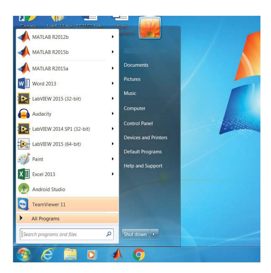
Figure 1.1: MATLAB appearance in the Windows Start bar.

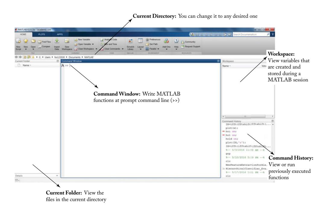
Figure 1.2: MATLAB interface window.

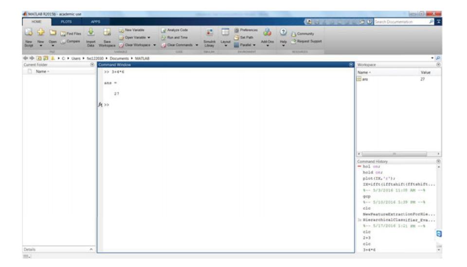
Figure 1.3: A simple computation in the Command Window.

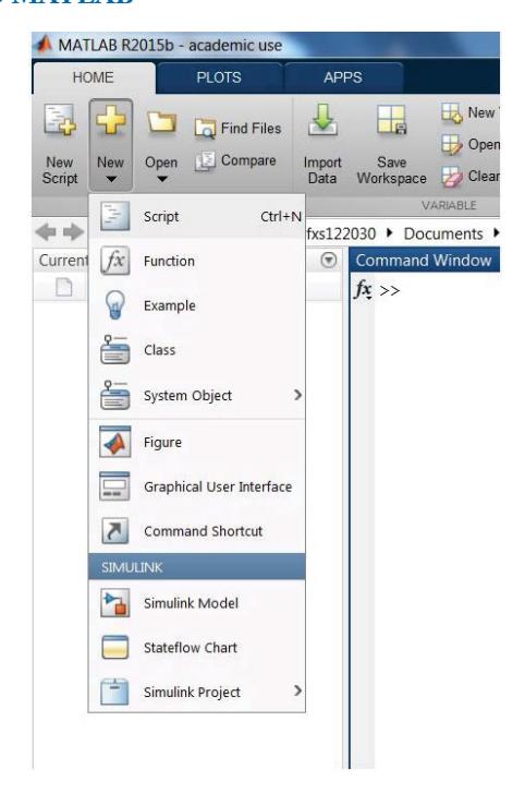
Figure 1.4: Starting a new m-file script in MATLAB.

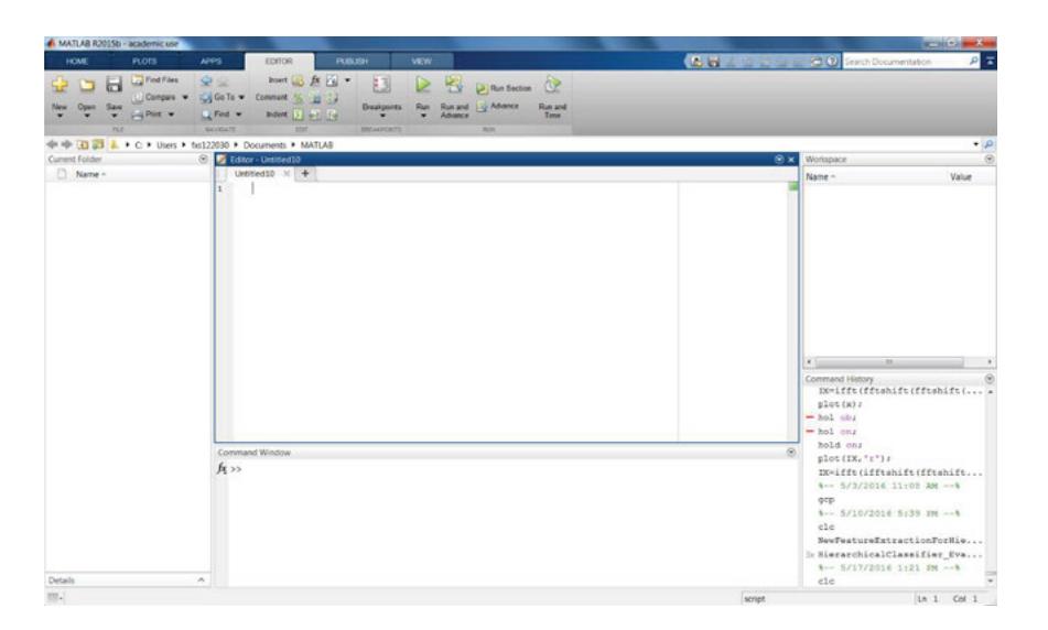
Figure 1.5: An m-file script docked in the EDITOR panel.

The following three operators work on an element-by-element basis:

.* multiplication of two vectors, element-wise
./ division of two vectors, element-wise
.^ raising all the elements of a vector to a power

As an example, to evaluate the expression $a^3 + sqrt{bd} – 4c$, where a = 1.2, b = 2.3, c = 4.5, and d = 4, type the following commands in the Command Window to get the answer (ans):

>> a=1.2:
>> b=2.3:
>> c=4.5;
>> d=4:
>> a^3+sqrt(b*d)-4*c
ans =
 -13.2388

Note the semicolon after each variable assignment. If the semicolon is omitted, the interpreter echoes back the variable value.

1.1.2 Vector Operations

Consider the vectors $mathbf{x} = [x_1, x_2, …, x_n]$ and $mathbf{y} = [y_1, y_2, …, y_n]$. The following operations indicate the resulting vectors:

$$x. * y = [x_1 y_1, x_2 y_2, …, x_n y_n]$$

$$x./y = left[frac{x_1}{y_1}, frac{x_2}{y_2}, …, frac{x_n}{y_n}right]$$

$$x. wedge p = [x_1^p, x_2^p, …, x_n^p].$$

Considering that the boldfacing of vectors/matrices are not used in .m files, in the notation adopted in this book, no boldfacing of vectors/matrices is shown to retain notation consistency with .m files.

The arithmetic operators + and – can be used to add or subtract matrices, vectors, or scalars. Vectors denote 1-dimensional arrays and matrices denote multi-dimensional arrays. For example:

>> x=[1,3,4]
>> y=[4,5,6]
>> x+y
ans=
5 8 10

In this example, the operator + adds the elements of the vectors x and y, element by element, assuming that the two vectors have the same dimension, in this case, or $1 times 3$ one row with three columns. An error occurs if one attempts to add vectors having different dimensions. The same applies for matrices.

To compute the dot product of two vectors (in other words, $sum_{i} x_{i} y_{i}$), use the multiplication operator ‘*’ as follows:

>> x*y'
ans =
43

Note the single quote after y denotes the transpose of a vector or a matrix.

An element-by-element multiplication of two vectors (or two arrays) is computed by the following operator:

>> x .* y
ans =
4 15 24

That is, $x cdot * y$ means $[1 times 4, 3 times 5, 4 times 6] = [4 quad 15 quad 24]$.

1.1.3 Complex Numbers

MATLAB supports complex numbers. The imaginary number is denoted with the symbol i or j, assuming that these symbols have not been used any other place in the program. It is critical to avoid such symbol conflicts for obtaining correct outcome. Enter the following and observe the outcomes:

>> z=3 + 4i % note the multiplication sign '*' is not needed after 4
>> conj(z) % computes the conjugate of z
>> angle(z) % computes the phase of z
>> real(z) % computes the real part of z
>> imag(z) % computes the imaginary part of z
>> abs(z) % computes the magnitude of z

One can also define an imaginary number with any other user-specified variables. For example, in the following manner:

>> img=sqrt(-1)
>> z=3 + 4*img
>> exp(pi*img)

1.1.4 ARRAY INDEXING

In m-files, all arrays (vectors) are indexed starting from 1; in other words, x(1) denotes the first element of the array x. Note that arrays are indexed using parentheses (.) and not square brackets [.] , as done in C/C++. To create an array featuring the integers 1–6 as elements, enter:

>> x=[1,2,3,4,5,6]

Alternatively, the notation ‘:’ can be used as follows:

>> x=1:6

This notation creates a vector starting from 1–6, in steps of 1. If a vector from 1–6 in steps of 2 is desired, then type:

>> x=1:2:6
ans =
  1 3 5

Additional examples are listed below:

>> ii=2:4:17
>> jj=20:-2:0
>> ii=2:(1/10):4

One can easily extract numbers in a vector. To concatenate an array, the example below shows how to use the operator ‘[ ]’ :

>> x=[1:3 4 6 100:110]

To access a subset of this array, type the following:

>> x(3:7)
>> length(x) % gives the size of the array or vector
>> x(2:2:length(x))

1.1.5 ALLOCATING MEMORY

Memory can get allocated for 1-dimensional arrays (vectors) using the command or function zeros . The following command allocates memory for a 100-dimensional array:

>> y=zeros(100,1);
>> y(30)
ans =
 0

The function zeros(n,m) creates an nm matrix with all 0 elements. One can allocate memory for 2-dimensional arrays (matrices) in a similar fashion. The command or function

>> y=zeros(4,5)

defines a 4 by 5 matrix.

Similar to the command zeros , the command ones can be used to define a vector containing all ones. For example,

>> y=ones(1,5)
ans=
 1 1 1 1 1

1.1.6 SPECIAL CHARACTERS AND FUNCTIONS

Some widely used special characters used in m-files are listed in Table 1.1. Some widely used functions are listed in Table 1.2.

Here is an example of the function length ,

>> x=1:10;
>> length(x)
ans =
 10

The function find returns the indices of a vector that are non-zero. For example, I = find(x>4) finds all the indices of x greater than 4. Thus, for the above example:

>> find(x>4)
ans =
  5 6 7 8 9 10

Table 1.1: Some widely used special characters used in m-files

Symbol	Meaning
pi	π (3.14)
^	indicates power (for example, 3^2 = 9)
NaN	not-a-number, obtained when encountering undefined operations, such as 0/0
Inf	represents +∞
;	indicates the end of a row in a matrix; also used to suppress printing on the screen (echo off )
%	comments—anything to the right of % is ignored by the .m file interpreter and is considered to be comments
‘	denotes transpose of a vector or a matrix; also used to define strings, for example, str1 = ‘DSP’
…	denotes continuation; three or more periods at the end of a line continue current function to next line

Table 1.2: Some widely used functions

Function	Meaning
sqrt	indicates square root, for example, sqrt(4) = 2
abs	absolute value, for example, abs(-3) = 3
length	length(x) gives the dimension of the array x
sum	finds sum of the elements of a vector
find	finds indices of nonzero

1.1.7 CONTROL FLOW

m-files have the following control flow constructs:

• if statements
• switch statements
• for loops
• while loops
• break statements

The constructs if , for , switch , and while need to terminate with an end statement. Examples are provided below:

if

>> x=-3;
if x>0
 str='positive'
elseif x<0
 str='negative'
elseif x== 0
 str='zero'
else
 str='error'
end

See the value of ‘str’ after running the above code.

while

x=-10;
while x<0
 x=x+1;
end

See the value of x after running the above code.

for loop

>>x=0;
for j=1:10
 x=x+j;
end

The above code computes the sum of all the numbers from 1–10.

break

With the break statement, one can exit early from a for or a while loop. For example,

>> x=-10;
while x<0
 x=x+2;
 if x == -2
  break;
 end
end

Some of the supported relational and logical operators are listed in Tables 1.3 and 1.4.

Table 1.3: Relational operators

Symbol	Meaning
<=	less than equal
<	less than
>=	greater than equal
>	greater than
==	equal
~=	not equal

Table 1.4: Logical operators

Symbol	Meaning
&	AND
~	NOT

1.1.8 PROGRAMMING IN MATLAB

Open a new script file as displayed in Figures 1.3 and 1.4. Save it first in a desired directory. Then write your MATLAB code and press Run button from the EDITOR panel. For instance, to write a program to compute the average (mean) of a vector x, the program should use the vector x as its input and return the average value. To write this program, follow the steps outlined below.

Type the following in an empty window:

x=1:10
L=length(x);
sum=0;
for j=1:L
sum=sum+x(j);
end
y=sum/L % the average of x

From the EDITOR panel, go to save ! Save As and enter average.m for the filename. Then click on the Run button to run the program. Figure 1.6 shows the MATLAB interactive window after running the program.

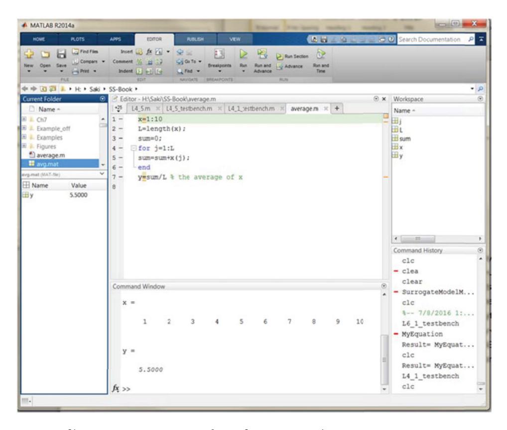
Figure 1.6: m-file script interactive window after running the program average.

1.1.9 SOUND GENERATION

Assuming the computer used has a sound card, one can use the function sound to play back speech or audio files through its speakers. That is, the function sound(y,FS) sends the signal in a vector y (with sample frequency FS) out to the speaker. Stereo sounds are played on platforms that support them, with y being an N-by-2 matrix.

Type the following code and listen to a 400 Hz tone:

>> t=0:1/8000:1;
>> x=cos(2*pi*400*t);
>> sound(x,8000);

Now generate a noise signal by typing:

>> noise=randn(1,8000); % generate 8000 samples of noise
>> sound(noise,8000);

The function randn generates Gaussian noise with zero mean and unit variance.

1.1.10 LOADING AND SAVING DATA

One can load or store data using the commands load and save . To save the vector x of the above code in the file data.mat, type:

>> save('data.mat', 'x')

To retrieve the data previously saved, type:

>> load data

The vector x gets loaded in memory. To see memory contents, use the command whos :

>> whos
Variable Dimension Type
x 1x8000 double array

The command whos gives a list of all the variables currently in memory, along with their dimensions and data type. In the above example, x contains 8,000 samples.

To clear up memory after loading a file, type clear all when done. This is important because, if one does not clear all the variables, conflicts can occur with other codes using the same variables.

1.1.11 READING WAVE AND IMAGE FILES

With MATLAB, one can read data from different file types (such as .wav, .jpeg, and .bmp) and load them in a vector.

To read an audio data file with .wav extension, use the following command:

>> [y,Fs]=audioread('filename')

This command reads a .wav file specified by the string filename and returns the sampled data in y with the sampling rate of Fs (in Hertz).

To read an image file, use the following command:

>> [y]=imread('filename')

This command reads a grayscale or color image from the string filename and returns the image data in the array y.

1.1.12 SIGNAL DISPLAY

Graphical tools are available in MATLAB to display data in a graphical form. Throughout the book, signals in both the time and frequency domains are displayed using the function plot,

This function creates a 2-D line plot of the data in y vs. corresponding x values.

1.2 MATLAB PROGRAMMING EXAMPLES

In this section, several simple MATLAB programs are presented.

1.2.1 SIGNAL GENERATION

In this example, we see how to generate and display continuous-time signals in the time domain. One can represent such signals as a function of time. For simulation purposes, a representation of time t is needed. Note that the time scale is continuous while computers handle operations in a discrete manner. Continuous time simulation is achieved by considering a very small time interval. For example, if a 1-s duration signal in millisecond (ms) increments (time interval of 0.001 s) is considered, then one sample every 1 ms or a total of 1,000 samples are generated for the entire signal leading to a continuous signal simulation. This continuous-time signal approximation or simulation is used in later chapters. It is important to note that a finite number of samples is involved in the simulation of a continuous-time signal, and thus to differentiate a continuous-time signal from a discrete-time signal, a much higher number of samples per second for a continuous-time signal needs to be used (very small time interval).

Figure 1.7 shows two continuous-time signals x1(t) and x2(t) with a duration of 3 s. By setting the time interval dt to 0.001 s, there is a total of 3,000 samples at $t = 0,0.001,0.002,0.003,ldots,2.999$ s. Note that throughout the book, the notations dt, delta, and $Delta$ are used interchangeably to denote the time interval between samples.

The signal x1(t) can be represented mathematically as follows:

$$x1(t) = begin{cases} 0 & 0 le t < 1 1 & 1 le t < 2 0 & 2 le t < 3 end{cases}$$
(1.1)

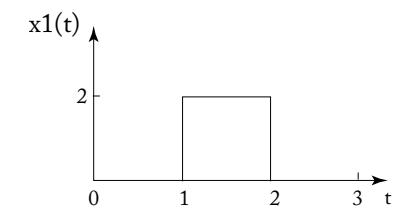
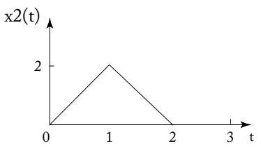
Figure 1.7: Continuous-time signals.

To simulate this signal, use the MATLAB functions ones and zeros. The signal value is zero during the first second, which means the first 1,000 samples are zero. This portion of the signal is simulated with the function zeros(1,1000). In the next second (next 1,000 samples), the signal value is 2, and this portion is simulated by the function 2*ones(1,1000). Finally, the third portion of the signal is simulated by the function zeros(1,1000). In other words, the entire duration of the signal is simulated by the following .m file function:

x1=[ zeros(1,1/dt) 2*ones(1,1/dt) zeros(1,1/dt)]

The signal x2(t) can be represented mathematically as follows:

$$x2(t) = begin{cases} 2t & 0 le t < 1 -2t + 4 & 1 le t < 2 0 & 2 le t < 3 end{cases}$$
(1.2)

A linearly increasing or decreasing vector can thus be used to represent the linear portions. The time vectors for the three portions or segments of the signal are 0:dt:1-dt, 1:dt:2-dt, and 2:dt:3-dt. The first segment is a linear function corresponding to a time vector with a slope of 2; the second segment is a linear function corresponding to a time vector with a slope of -2 and an offset of 4; and the third segment is simply a constant vector of zeros. In other words, the entire duration of the signal for any value of dt can be simulated by the following .m file function:

x2=[2*(0:dt:(1-dt)) -2*(1:dt:(2-dt))+4 zeros(1,1/dt)]

Figures 1.8 and 1.9 show the MATLAB code and the plot of the above signal generation, respectively. Signals can be displayed using the function plot(t,data). For proper plotting, first the correct t vector needs to be generated. Here this is done by using the function linspace:

>> t=linspace(0,E,N)

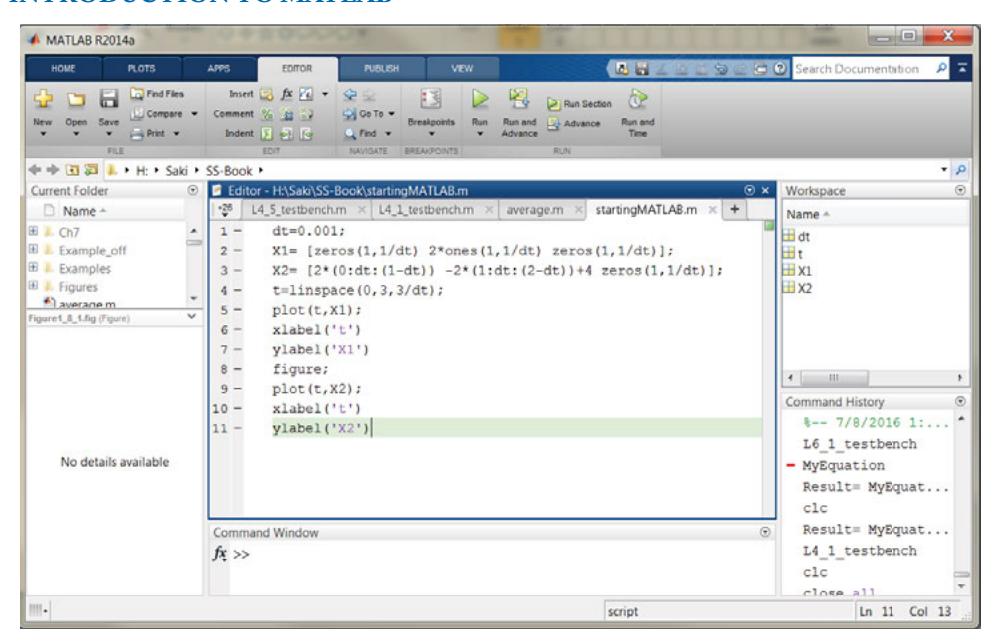
Figure 1.8: MATLAB code of a signal generation example.

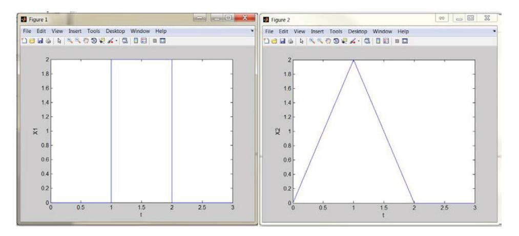
Figure 1.9: Signal plots.

This function generates a vector t of N points linearly spaced between and including 0 and E , where N is equal to E/dt .

1.2.2 Generating a Periodic Signal

In this example, a simple periodic signal is generated. This example involves generating a periodic signal in textual mode and displaying it graphically. The shape of the signal ( sin , square , triangle , or sawtooth ) can be modified, as well as its frequency and amplitude, by using appropriate control parameters. The MATLAB code and the plots generated by it are shown in Figures 1.10 and 1.11, respectively.

Now consider an m-file code to generate four types of waveforms using the functions sin , square , and sawtooth . To change the amplitude and frequency of the waveforms, two control parameters named Amplitude ( A ) and Frequency ( f ) are used. Waveform Type ( w ) is another parameter used for controlling the waveform type. With this control parameter, one can select from multiple inputs. Finally, the waveforms are displayed by using the function plot .

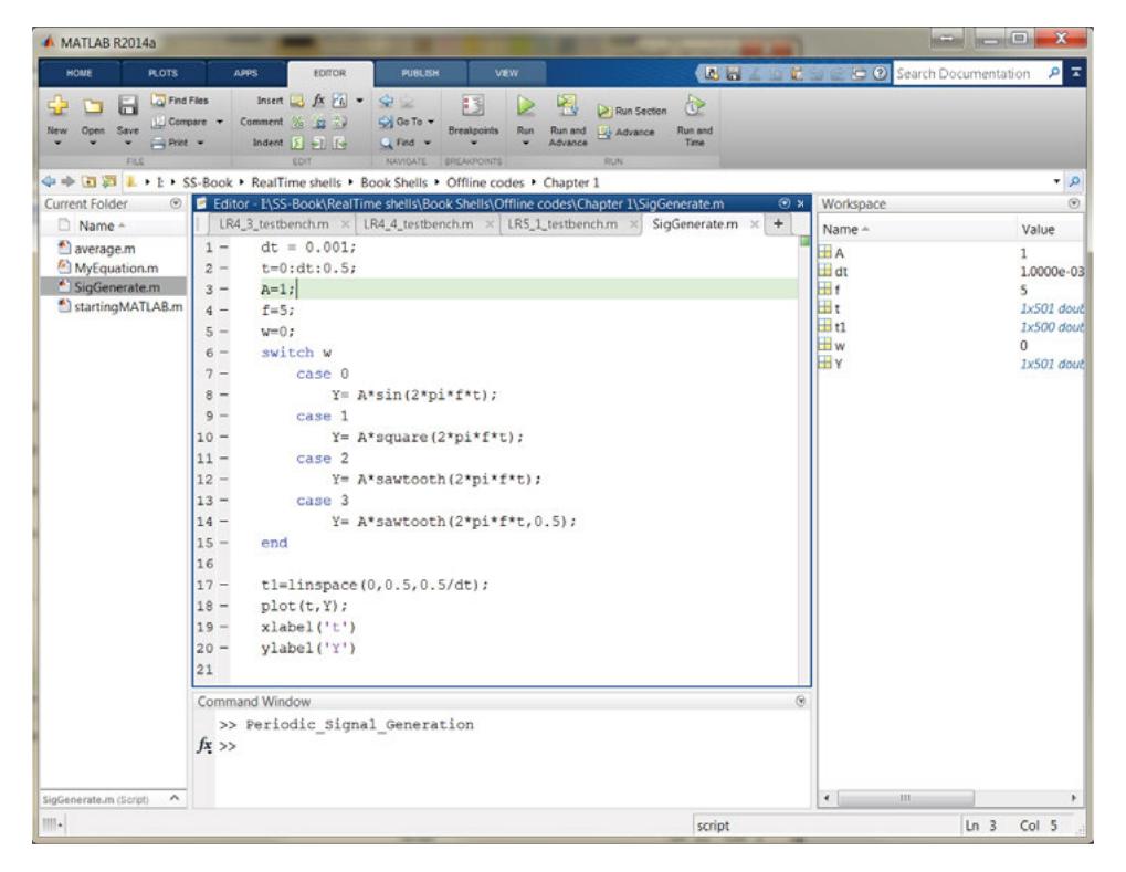
Figure 1.10: Periodic signal generation example.

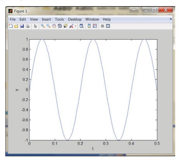
Figure 1.11: Plot of a periodic sinusoid signal.

1.3 Lab Exercises

1. Write an m-file code to add all the numbers corresponding to the even indices of an array. For instance, if the array x is specified as x = [1, 3, 5, 10], then 13 (= 3 + 10) should be returned. Use the program to find the sum of all even integers from 1–1,000. Run your code. Also, rewrite the code where x is the input vector and y is the sum of all the numbers corresponding to the even indices of x.
2. Explain the operation performed by the following .m file:

L=length(x);
for j=1:L
if x(j) < 0
x(j)=-x(j);
end
end

Rewrite this program without using a for loop.

3. Write an .m file code that implements the following hard-limiting function:

$$x(t) = begin{cases} 0.2 & t ge 0.2 -0.2 & t < 0.2 end{cases}$$
(1.3)

For t, use 1,000 random numbers generated by using the function rand .

4. Write a MATLAB code to generate two sinusoid signals with the frequencies f1 Hz and f2 Hz and the amplitudes A1 and A2, based on a sampling frequency of 8,000 Hz with the number of samples being 256. Set the frequency ranges from 100–400 Hz and set the amplitude ranges from 20–200. Generate a third signal with the frequency f3 = (mod (lcm (f1, f2), 400) + 100) Hz, where mod and lcm denote the modulus and least common multiple operation, respectively, and the amplitude A3 is the sum of the amplitudes A1 and A2. Use the same sampling frequency and number of samples as specified for the first two signals. Display all the signals using the legend on the same waveform graph and label them accordingly.

Software Development Tools

This chapter covers the steps that are required in order to install the software tools for running C codes on Android and iPhone smartphones. Later in Chapter 3, it will be shown how to convert MATLAB codes to C codes.

The Android development environment used here is the IntelliJ IDEA-based Android Studio Bundle (Android Studio). C codes are made available to the Android Java environment through the use of the Java Native Interface ( JNI) wrapper. Thus, it is also necessary to install the Android Native Development Kit (NDK). This development kit allows one to write C codes, compile, and debug them on an emulated Android platform or on an actual Android smartphone/tablet.

Screenshots are used to show the steps and configuration options involved in the installation when using the Windows operating system. The same software tools are also available for other operating systems.

2.1 Android Tools Installation Steps

This section covers the installation of the necessary software packages for Android app development. Start by creating a directory where the tools are to be installed. A generic directory of C:Android is used here and the setup is done such that all Android development related files are placed within the C:Android directory. Before running Android Studio, the latest Java JDK needs to be installed.

2.1.1 Java JDK

If the Java Development Kit ( JDK) is not already installed on your computer, or you do not have the latest version, download it from Oracle’s website and follow the installation steps indicated by the installer. The latest JDK package at the time of this writing can be found on Oracle’s website at:

http://www.oracle.com/technetwork/java/javase/downloads/index.html

Click on the JDK Download button in the Java Platform, Standard Edition section and you will be taken to the page shown in Figure 2.1. From the list of supported platforms, select the correct version for your operating system. For example, if you are running a 64-bit operating system, select the appropriate package.

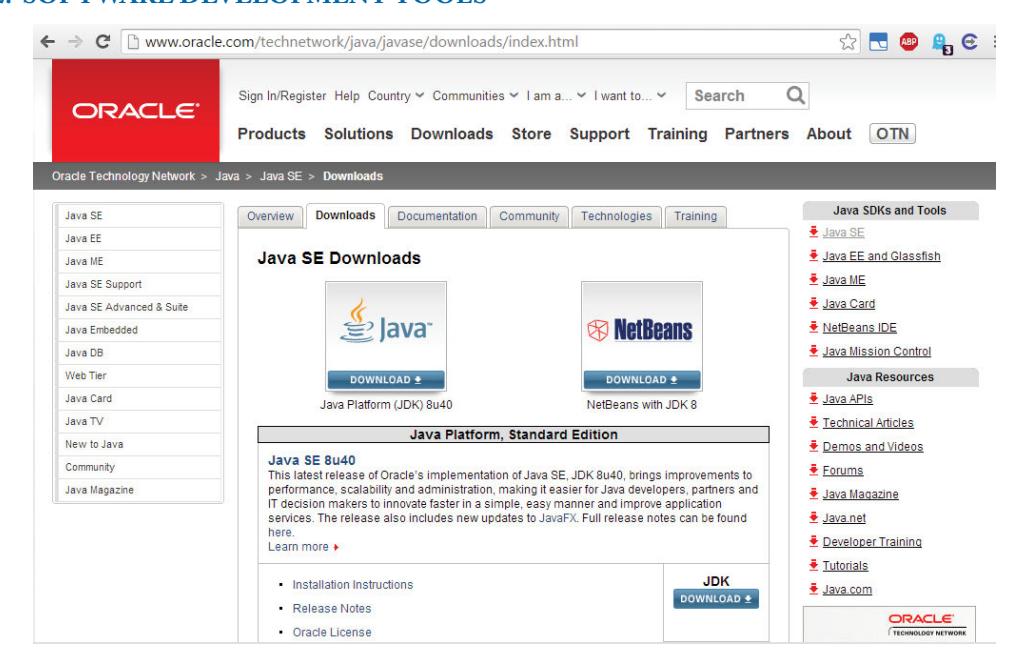
Figure 2.1: Java installation.

2.1.2 Android Studio Bundle and Native Development Kit

The most recent versions of Android Studio and the NDK at the time of this writing are used to run the lab experiments in this book. For the Windows, Mac, and Linux installation, the Android Studio Bundle is available as an executable installer which incorporates both the development environment and Android SDK tools.

The NDK can be downloaded and installed from within Android Studio: http://developer.android.com/studio/index.html.

Download the Android Studio installation executable and run the Android Studio installer. For platform specific instructions, the installation instructions appear at https://developer.android.com/studio/install.html.

During the installation of Android Studio, there are two important settings that are critical to be performed correctly; see Figures 2.2 and 2.3. For the setting shown in Figure 2.2, make sure that all the components are selected for installation, and, for the setting shown in Figure 2.3, make sure that Android Studio and Android SDK are installed in the directory C:Android. To do so, manually create the directories by using the Browse option and create a Studio folder and an sdk folder. When the installer is finished, Android Studio can get started. Then, the Android Studio Setup Wizard is to be activated which is covered next. The Android NDK can be downloaded and installed from within Android Studio.

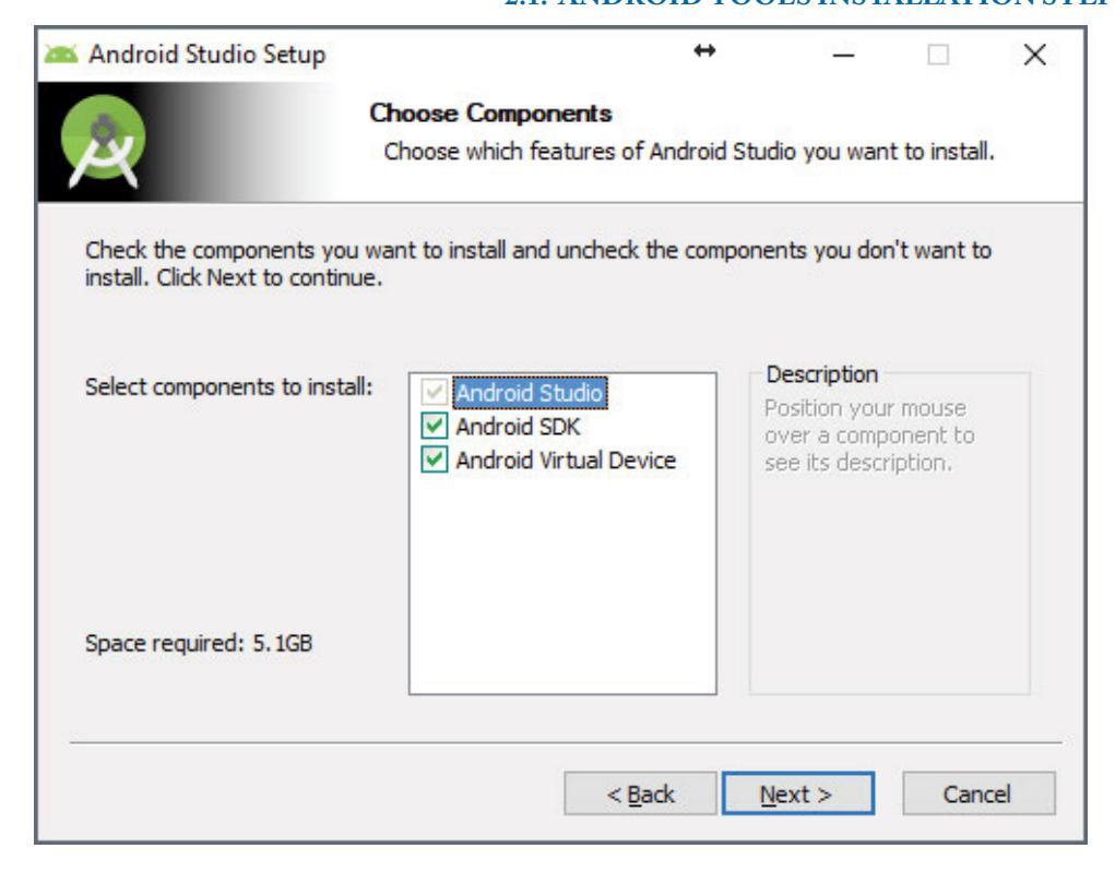
Figure 2.2: Android Studio Setup.

2.1.3 Android Studio Setup Wizard

When Android Studio completes its installation, make sure the checkbox to run Android Studio is checked. The Android Studio Setup Wizard begins. Follow the steps noted below.

• Hit next on the Welcome Screen.
• Select Custom to finish the configuration as displayed in Figure 2.4.
• Select your preferred UI Theme IntelliJ or Darcula.
• Make sure all boxes are checked under Android SDK, Performance (HAXM), and AVD.
• – Make sure to select the SDK Location as noted above, that is C:Androidsdk.
• Use the recommended Emulator Settings.
• Review your settings and hit Finish.

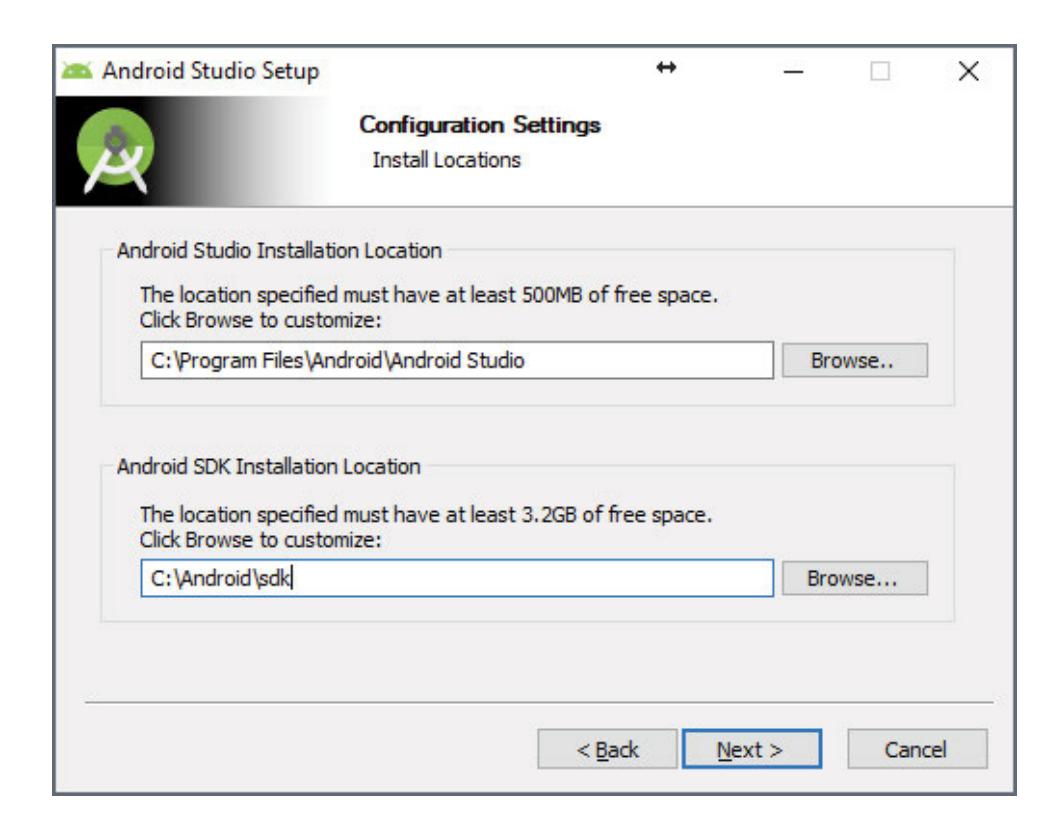
Figure 2.3: Configuration settings.

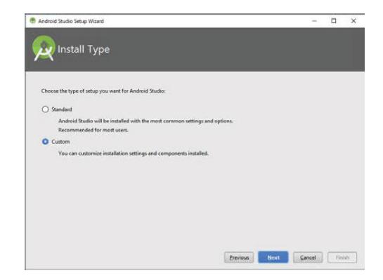
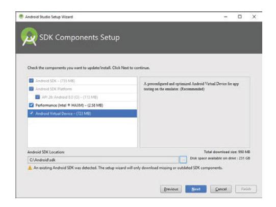
Figure 2.4: Custom installation. Figure 2.5: SDK component setup.

When this is done, the Android Studio home screen should appear as shown in Figure 2.6. Now run the SDK Manager, whose entry can be found by clicking on the Configure option. From this menu, additional system images for emulation and API packages for future Android versions can get added. Select any Android API level you may require listed on the SDK Platform tab; see Figure 2.7. On the SDK Tools tab, check the CMake, LLDB, NDK tools; see Figure 2.8. Click on Apply and follow the steps.

Allow the update process to complete.

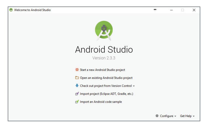
Figure 2.6: Android Studio home screen.

2.1.4 Android Emulator Configuration

The last item to take care of is configuring an Android Virtual Device (AVD) Tools menu (see Figure 2.9) and select the Manage AVDs option to open the Android Virtual Device Manager as shown in Figure 2.10. By default, Android Studio creates an x86 AVD. Since our development focus is ARM-based implementation, an ARM-based emulator instance is required. Begin by deleting any existing AVD instances.

Click the Create… button to start configuring the AVD (see Figure 2.11). Use a descriptive name such as Android_5.1.1 or whatever the target of the AVD is. For the Device option, select a device with a good screen resolution for your computer—Nexus S is usually fine. For compatibility with newer smartphones, it is suggested to select the Target as the latest available version with the CPU/ABI as ARM (armeabi-v7a). RAM allocation does not need to be large so choose the 512 MB amount. Last, set the SD Card and Internal Storage size to 256 MB. The Snapshot option is useful to select as it normally takes a long time for the AVD to boot. The snapshot will save the memory state of the emulator to your hard drive so that starting the emulator occurs much faster.

2. SOFTWARE DEVELOPMENT TOOLS

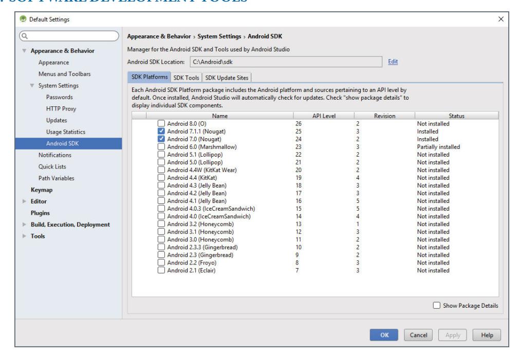
Figure 2.7: SDK manager.

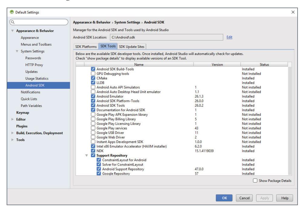
Figure 2.8: SDK tools.

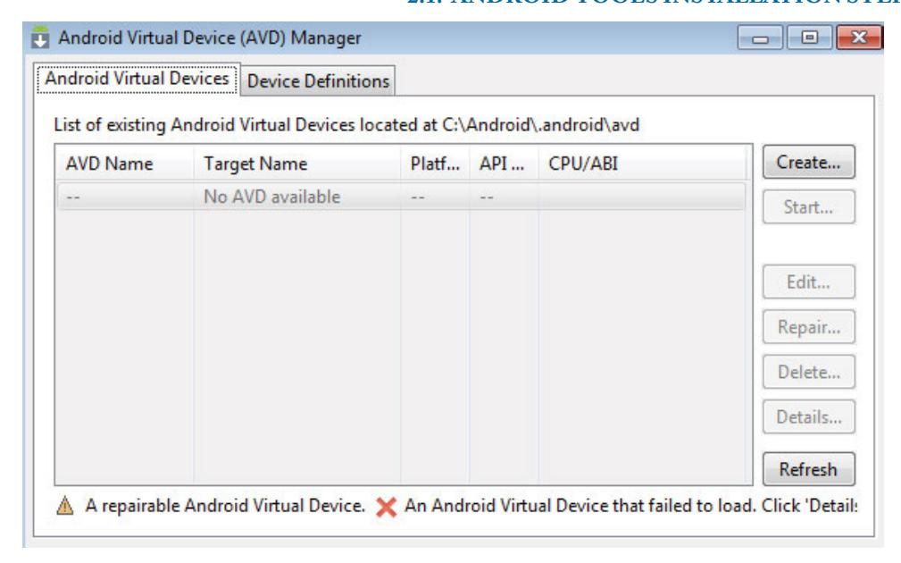
Figure 2.9: Android virtual device.

You should now be able to create the AVD by clicking OK. Select the AVD you just created in the list of devices and click the Start option (see Figure 2.12). For the first launch of the AVD, it is best to select the Wipe user data and Save to snapshot options (see Figure 2.12). Click Launch and wait for the AVD to boot. Once the AVD launches, unlock the screen and delete the greeting message. Open the apps menu and do the same with the message that appears there. Go back to the home screen and close the emulator. In the AVD Manager, select the Start option for your AVD again. This time, make sure that only the Launch from snapshot box is checked in the Launch Options menu. Click Launch and the emulator should boot significantly faster than it booted previously.

Expand the Defaults listing and select the Android Application option. Under the General tab, scroll down to the Target Device section and select the Show chooser dialog option. Next, switch to the Emulator tab and enter the text -no-snapshot-save in the field marked

AVD Name:	Android_5.1.1
Device:	Nexus S (4.0”, 480 × 800: hdpi) ▼
Target:	Android 5.1.1 – API Level 22 ▼
CPU/ABI:	ARM (armeabi-v7a) ▼
Keyboard:	✓ Hardware keyboard present
Skin:	Skin with dynamic hardware controls
Front Camera:	None ▼
Back Camera:	None
Memory Options:	RAM: 512 VM Heap: 32
Internal Storage:	256	MiB ▼
SD Card:
	Size: 256	MiB ▼
	⊚ File:	Browse
Emulation Options:	✓ Snapshot	Use Host GPU
Override the existing AVD with the same name

Figure 2.10: AVD creation.

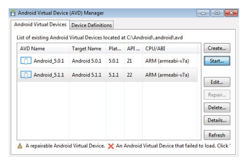
Figure 2.11: AVD manager.

	ity: High (240) Scale display to real	size
	Screen Size (in):	4.0
	Monitor dpi:	96	?
	Scale:	default
_	Scale: Wipe user data Launch from snapshot
	Save to snapshot

Figure 2.12: Launch options.

Additional command line options and ensure that the checkbox is enabled (see Figure 2.14). Repeat these steps for the Android Tests section as well. Later on when apps are being installed onto the emulator, this will ensure that the emulator does not retain the old app data and remains clean.

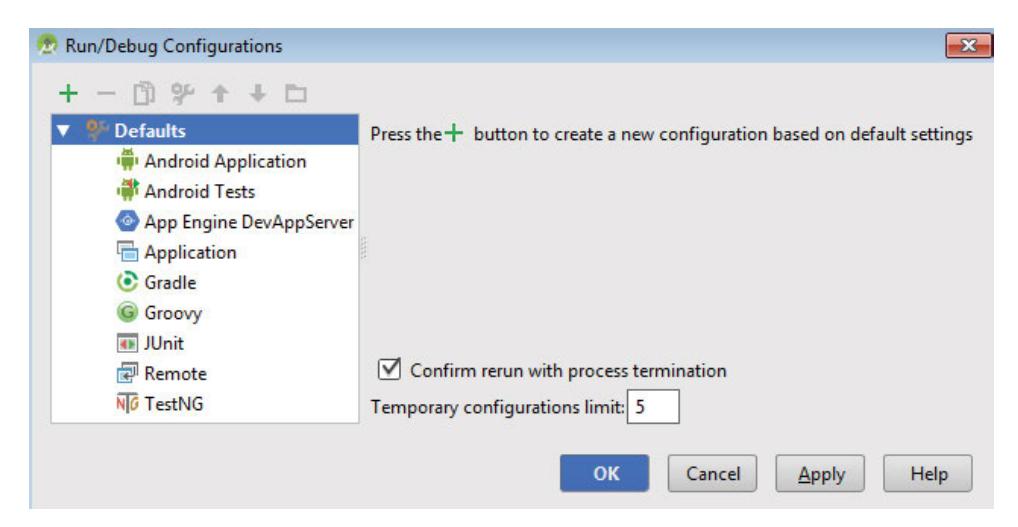
Figure 2.13: Run configurations.

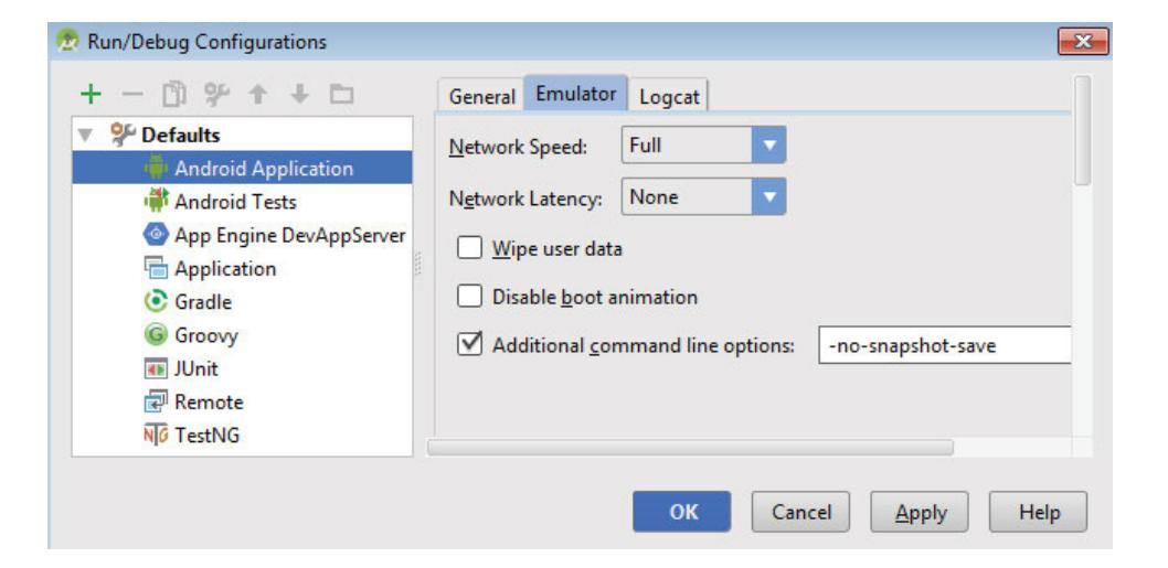
Figure 2.14: Emulator configurations.

2.1.5 GETTING FAMILIAR WITH ANDROID SOFTWARE TOOLS

This lab covers the creation of a simple app on the Android smartphone platform by constructing a “Hello world!” program. Android Studio and NDK tools are used for code development, emulation, and code debugging. All the codes needed for this and other labs can be extracted from the software package mentioned in the preface. Start by launching Android Studio, and, if not already done, set up an Android Virtual Device (AVD) for use with the Android emulator.

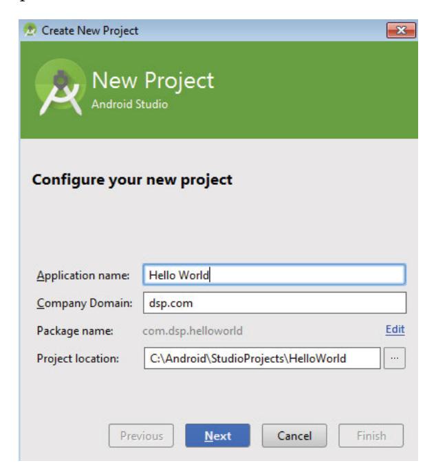
Figure 2.15: Initial screen of Android Studio.

• Begin by creating a new Android project using the Quick Start menu found on the Android Studio home screen.
• Set the Application Name to HelloWorld and the project location to a folder within the C:Android directory.
• Change the Company Domain to an appropriate domain, for example, utdallas.edu so that the package name reads as utdallas.edu.helloworld . This is of importance later, as it will affect the naming of your native code methods. Refer to Figure 2.15 for the previous three steps.

• The Target Android device should be set to Phone and Tablet using a Minimum SDK setting of API 15 .

• Click Next and on the following screen choose to create an Empty Activity .

• Click Next again to create an Empty Activity and leave the default naming.
• Select Finish. The new app project is now created and the main app editor will open to show the GUI layout of the app.
• Navigate to the java directory of the app in the Project window and open the MainActivity.java file under com.dsp.helloworld.

The entity that typically defines an Android app is called an Activity. Activities are generally used to define user interface elements. An Android app has activities containing various sections that users might interact with, such as the main app window. Activities can also be used to construct and display other activities—such as if a settings window is needed. Whenever an Android app is opened, the onCreate function or method is called. This method can be regarded as the “main” (C terminology) of an activity. Other methods may also be called during various portions of the app lifecycle as detailed at the following website:

http://developer.android.com/training/basics/activity-lifecycle/starting.html

In the default code created by the SDK, setContentView(R.layout.activity_main) exhibits the GUI. The layout is described in the file res/layout/activity_main.xml in the Package Explorer window. Open this file to preview the user interface. Layouts can be modified using the WYSIWYG editor, which is built into Android Studio. For now, the basic GUI suits our purposes with one minor modification noted below.

• Open the XML text of the layout (see Figure 2.16) by double clicking on the Hello world! text or by clicking on the activity_main.xml tab next to the Graphical Layout tab.
• Add the line android:id=”@+id/Log” within the section on a new line and save the changes. This gives a name to the TextView UI element.

TextView in the GUI acts similar to a console window. It displays text. Additional text can be appended by adding the android:id directive to TextView code.

After setting up the emulator and the app GUI, let us cover interfacing with C codes. Note that it is not required to know the Java code syntax. The purpose is to show that the Java Native Interface ( JNI) is a bridge between Java and C codes. Java is useful for handling Android APIs for sound and video i/o, whereas the signals and systems codes are done in C. Note that to conduct the labs, the programming is not done in C, and C codes are generated by the MATLAB Coder discussed in the next chapter.

A string returned from a C code is examined next. The procedure to integrate native code consists of creating a C code segment and performing alterations to the project. First, it is

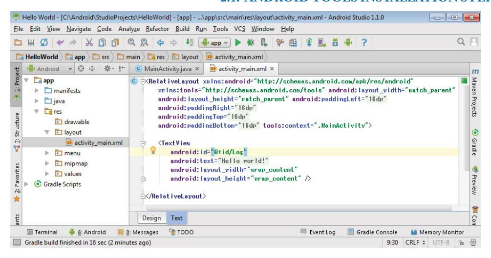
Figure 2.16: Hello World app.

required to add support for the native C code to the project. The first step is to create a folder in which the C code will be stored. In the Project listing, navigate down to New ! Folder ! JNI to create a folder in the listing called jni. Refer to Figures 2.17–2.20. Figure 2.19 shows how the Project listing view may be changed in order to show the jni folder in the main source listing.

Android Studio now needs to be configured to build a C code using the Gradle build utility. Begin by specifying the NDK location in the project local.properties file according to Figure 2.21. Assuming the directory C:/Android is used for setting up the development tools, the location specification would be as follows:

ndk.dir=C:\Android\ndk

Next, the native library specification needs to get added to the build.gradle file within the project listing under the “app” folder. This specification declares the type of external build and its configuration file which defines the name of the external library that Java will load. This is done by adding the following code within the android section:

externalNativeBuild {
   cmake {
      path "CMakeLists.txt"
   }
}

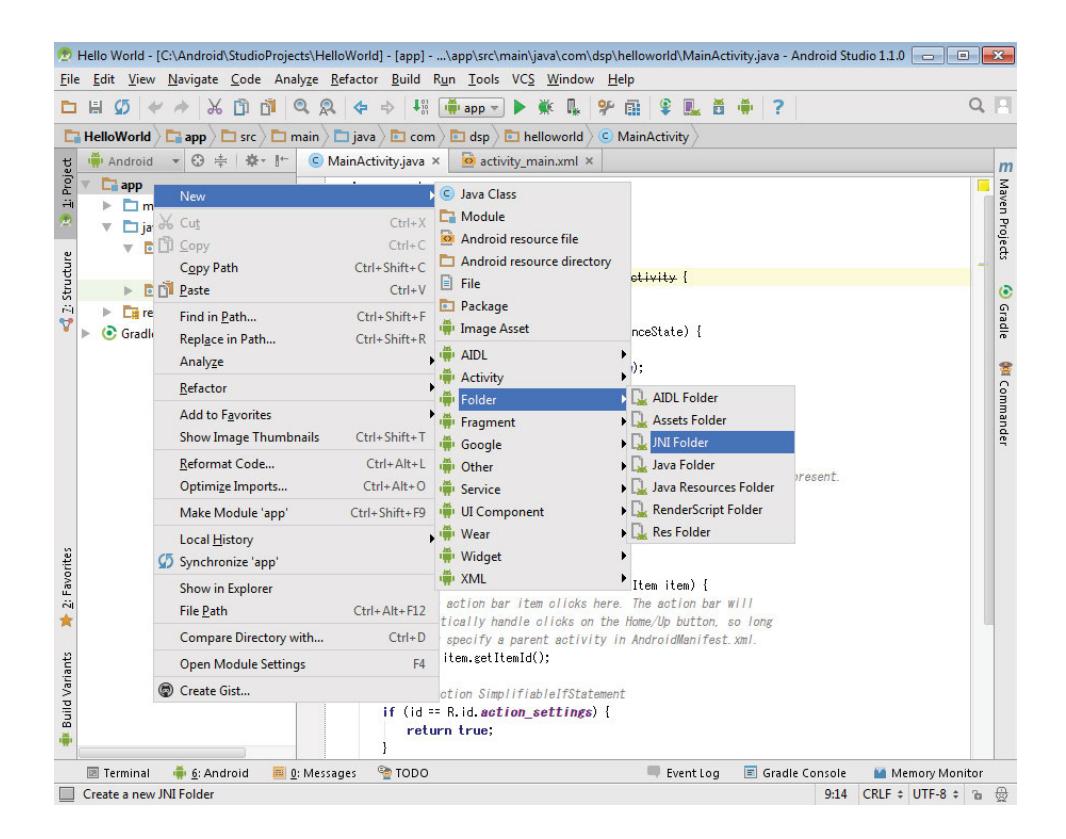
Figure 2.17: JNI folder.

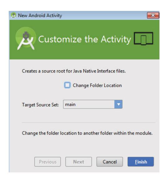
Figure 2.18: New Android activity.

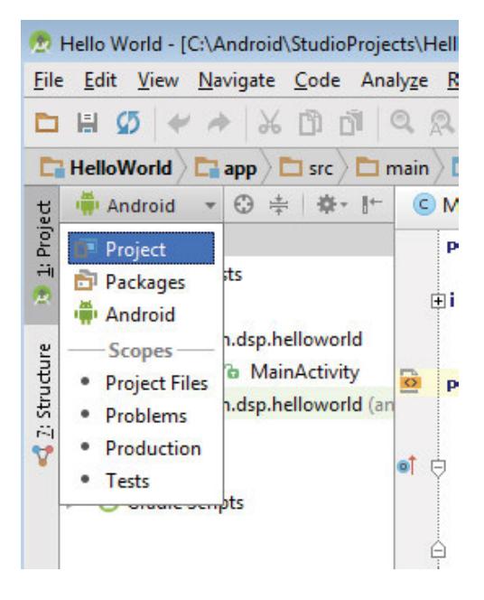
Figure 2.19: Project listing.

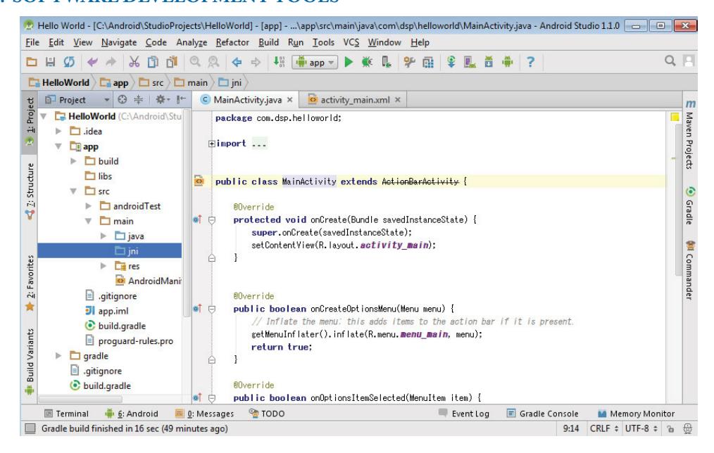
Figure 2.20: MainActivity.java.

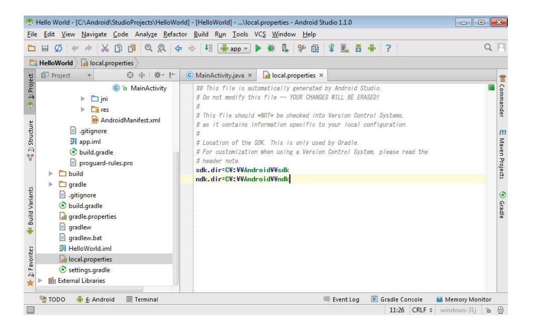
Figure 2.21: local.properties.

The correct placement of the code is highlighted in Figure 2.22.

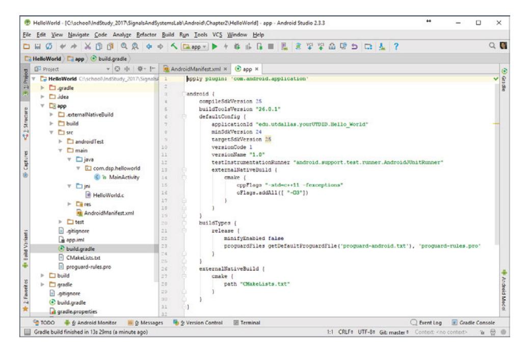
Figure 2.22: Code placement.

Integrating C Code with Android JNI

The C code considered here consists of a simple method to return a string when it is called from the onCreate method. First, the code that defines the native method needs to be included. Create a new HelloWorld.c file. Add the following code and save the changes:

#import <jni.h>
jstring Java_com_dsp_helloworld_MainActivity_getString
   (JNIEnv* env, jobject thiz ) {
             return (*env)->NewStringUTF(env, "Hello UTD!");
}

This code defines a method that returns a Java string object according to the JNI specifications with the text “Hello UTD!”. The naming for this method is dependent on what is called the fully qualified name of the native method, which is defined in MainActivity. There are alternate methods of defining native methods that will be discussed in later labs.

Next, the native method needs to be declared within MainActivity.java (see Figure 2.23) according to the naming used in the C code. To do so, add this declaration below the onCreate method already defined.

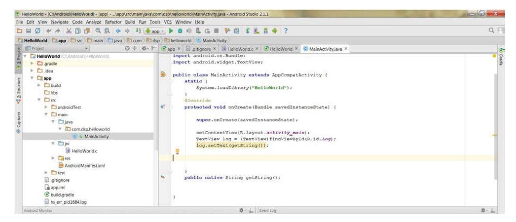
Figure 2.23: TextView GUI object representation.

public native String getString();

Next, add the following code within the public class to load the native library:

static {
       System.loadLibrary("HelloWorld");
}

To use the TextView GUI object, it needs to be imported by adding the following declaration to the top of the MainActivity.java file:

import android.widget.TextView;

The TextView defined in the GUI layout needs to be hooked to the onCreate method by adding the following lines to the end of the onCreate method code section (after setContentView but inside the bracket):

TextView log = (TextView) findViewById(R.id.Log);
log.setText( getString() );

This will cause the text displayed in the TextView to be changed by the second line which calls the C getString method.

Save the changes and select the Make Project option (located under the Build category on the main toolbar). Android Studio would display the build progress and notify if any errors occur. Next, run the app on the Android emulator using the Run app option located in the Run menu of the toolbar. If an emulator is already running, an option will be given to deploy the app to the selected device (see Figure 2.24). Android Studio should launch the emulator and the screen (see Figure 2.25) would display “Hello UTD!”. To confirm that the display is being changed, comment out the line log.setText() and run the app again. This time the screen would display “Hello World!”.

Adding LogCat Logging

Note that the LogCat is equivalent to the main system log or display of the execution information. Here, the code from the previous project is modified to enable the log output capability as follows:

• Add the logging library to the build.gradle file (see Figure 2.22) by adding the line ldLibs "log" to the ndk section that was added previously.
• Add the Android logging import to the top of the HelloWorld.c source file (see Figure 2.26) by adding the line #include<android/log.h>.
• Add the following code to output the test message before the return statement:

int classNum = 9001;
int secNum = 1;
__android_log_print(ANDROID_LOG_ERROR, "HelloWorld", "DSP %d.%03d",
      classNum, secNum);

The __android_log_print() method (two underscores at the beginning) is similar to the printf function in C. The first two parameters are the log level and the message tag. In the above example, the string has a specified integer for the class number inserted, followed by a specified integer for the section number. The same number formatting that is possible when using the printf function may also be used here. For instance, the section number can be formatted to three characters width with leading zeros. Variables are last and are inserted with the formatting specified in the message string in the order they are listed.

Save the changes made to the HelloWorld.c source file and run the app again. This time, Android Studio should automatically open the Android DDMS window and show the LogCat screen. The message “DSP 9001.001” would appear in the listing if the previous procedures were performed properly (see Figure 2.26).