1.4.1 Causal representation learning

Many state-of-the-art deep learning methods attempt to learn geometric representations of the objects being modeled. However, these methods struggle with learning causally meaningful representations. For example, consider a video of a child holding a helium-filled balloon on a string. Suppose we had a corresponding vector representation of that image. If the vector representation were causally meaningful, then manipulating the vector to remove the child and converting the manipulated vector to a new video would result in a depiction of the balloon rising upwards. Causal representation learning is a promising area of deep representation learning that’s still in its early stages. This book provides several examples in different chapters of causal models built upon deep learning architectures, providing an introduction to the fundamental ideas used in this exciting new growth area of causal AI.

1.4.2 Causal reinforcement learning

In canonical reinforcement learning, learning agents ingest large amounts of data and learn like Pavlov’s dog; they learn actions that correlate positively with good outcomes and negatively with bad outcomes. However, as we all know, correlation does not imply causation. Causal reinforcement learning can highlight cases where the action that causes a higher reward differs from the action that correlates most strongly with high rewards. Further, it addresses the problem of credit assignment (correctly attributing rewards to actions) with counterfactual reasoning (i.e., asking questions like “how much reward would the agent have received had they been using a different policy?”). Chapter 12 is devoted to causal reinforcement learning and other areas of causal decision-making.

1.4.3 Large language models and foundation models

Large language models (LLMs) such as OpenAI’s GPT, Google’s Gemini, and Meta’s Llama are deep neural language models with many billions of parameters trained on vast amounts of text and other data. These models can generate highly coherent natural language, code, and content of other modalities. They are foundation models, meaning they provide a foundation for building more domain-specific machine learning models and products. These products, such as Microsoft 365 Copilot, are already having a tremendous business impact.

A new area of investigation and product development investigates LLMs’ ability to answer causal questions and perform causal analysis. Another line of investigation is using causal methods to design and train new LLMs with optimized causal capabilities. In chapter 13, we’ll explore the intersection of LLMs and causality.

1.5 A machine learning-themed primer on causality

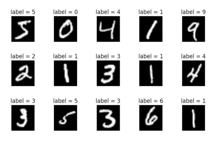
Now that you’ve seen the many ways that causal inference can improve machine learning, let’s look at the process of incorporating causality into AI models. To do this, we will use a popular benchmark dataset often used in machine learning: the MNIST dataset of images of handwritten digits, each labeled with the actual digit represented in the image. Figure 1.4 illustrates multiple examples of the digits in MNIST.

{alt=”Examples of handwritten digits from the MNIST dataset, showing various styles of digits 0 through 9.”}

Figure 1.4 Each image in the MNIST dataset is an image of a written digit, and each image is labeled with the digit it represents.

MNIST is essentially the “Hello World” of machine learning. It is primarily used to experiment with different machine learning algorithms and to compare their relative strengths. The basic prediction task is to take the matrix of pixels representing each image as input and return the correct image label as output. Let’s start the process of incorporating causal thinking into a probabilistic machine learning model applied to MNIST images.

1.5.1 Queries, probabilities, and statistics

First, we’ll look at the basic process without including causal inference. Machine learning can use probability in analyses about quantities of interest. To do so, a probabilistic machine learning model learns a probabilistic representation of all the variables in that system. We can make predictions and decisions with probabilistic machine learning models using a three-step process.

1. Pose the question—What is the question you want to answer?
2. Write down the math—What probability (or probability-related quantity) will answer the question, given the evidence or data?
3. Do the statistical inference—What statistical analysis will give you (or will estimate) that quantity?

There is more formal terminology for these steps (query, estimand, and estimator) but we’ll avoid the jargon for now. Instead, we’ll start with a simple statistical example problem. Your step 1 might be “How tall are Bostonians?” For step 2, you might decide that knowing the mean height (in probability terms, the “expected value”) of everyone who lives in Boston will answer your question. Step 3 might involve randomly selecting 100 Bostonians and taking their average height; statistical theorems guarantee that this sample average is a close estimate of the true population mean.

Let’s extend that workflow to modeling MNIST images.

STEP 1: POSE THE QUESTION

{alt=”A handwritten digit that could be interpreted as either a 4 or a 9, illustrating an MNIST classification challenge.”}

Figure 1.5 Is this an image of the digit 4 or 9? The canonical task of the MNIST dataset is to classify the digit label given the image.

Suppose we are looking at the MNIST image in figure 1.5, which could be a “4” or could be a “9”. In step 1, we articulate a question, such as “given this image, what is the digit represented in this image?”

STEP 2: WRITE DOWN THE MATH

In step 2, we want to find some probabilistic quantity that answers the question, given the evidence or data. In other words, we want to find something we can write down in probability math notation that can answer the question from step 1. For our example with figure 1.5, the “evidence” or “data” is the image. Is the image a 4 or a 9? Let the variable I represent the image and D represent the digit. In probability notation, we can write the probability that the digit is a 4, given the image, as P(D=4|I= ), where I= is shorthand for I being equal to some vector representation of the image. We can compare this probability to P(D=9|I= ), and choose the value of D that has the higher probability. Generalizing to all ten digits, the mathematical quantity we want in step 2 is shown in figure 1.6.

$$argmax P(D=d|I=P)$$

Figure 1.6 Choose the digit with the highest probability, given the image.

In plain English, this is “the value d that maximizes the probability that D equals d, given the image,” where d is one of the ten digits (0–9).

STEP 3: DO THE STATISTICAL INFERENCE

Step 3 uses statistical analysis to assign a number to the quantity we identified in step 2. There are any number of ways we can do this. For example, we could train a deep neural network that takes in the image as an input and predicts the digit as an output; we could design the neural net to assign a probability to D=d for every value d.

1.5.2 Causality and MNIST

So how could causality feature in the previous section’s three-step analysis? Yann LeCun is a Turing Award winner (computer science’s equivalent of the Nobel prize) for his work on deep learning, and he’s director of AI research at Meta. He is also one of the three researchers behind the creation of MNIST. He discusses the causal backstory of the MNIST data on his personal website, https://yann.lecun.com/exdb/mnist/index.html:

The MNIST database was constructed from NIST’s Special Database 3 and Special Database 1 which contain binary images of handwritten digits. NIST originally designated SD-3 as their training set and SD-1 as their test set. However, SD-3 is much cleaner and easier to recognize than SD-1. The reason for this can be found on the fact that SD-3 was collected among Census Bureau employees, while SD-1 was collected among high-school students. Drawing sensible conclusions from learning experiments requires that the result be independent of the choice of training set and test among the complete set of samples. Therefore, it was necessary to build a new database by mixing NIST’s datasets.

In other words, the authors mixed the two datasets because they argue that if they trained a machine learning model solely on digits drawn by high schoolers, it would underperform when applied to digits drawn by bureaucrats. However, in real-world settings, we want robust models that can learn in one scenario and predict in another, even when those scenarios differ. For example, we want a spam filter to keep working when the spammers switch from Nigerian princes to Bhutanese princesses. We want our self-driving cars to stop even when there is graffiti on the stop sign. Shuffling the data like a deck of cards is a luxury not easily afforded in real-world settings.

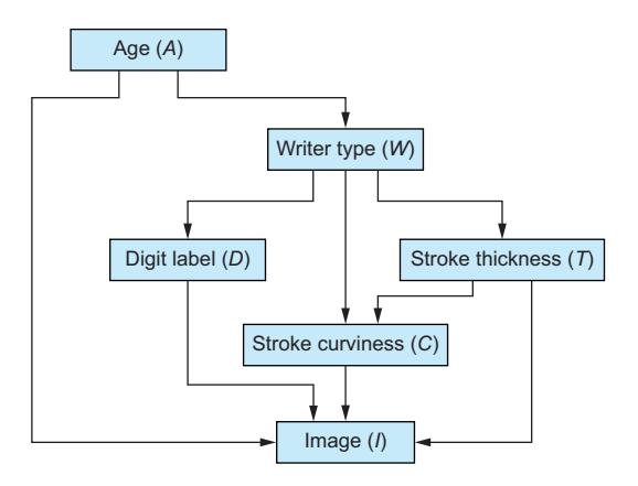
Causal modeling leverages knowledge about the causal mechanisms underlying how the digits are drawn that will help models generalize beyond high school students and bureaucrats in the training data to high schoolers in the test data. Figure 1.7 illustrates a causal DAG representing this system.

This particular DAG imagines that the writer determines the thickness and curviness of the drawn digits, and that high schoolers tend to have a different handwriting style than bureaucrats. The graph also assumes that the writer’s classification is a cause of what digits they draw. Perhaps bureaucrats write more 1s, 0s, and 5s, as these

{alt=”A causal Directed Acyclic Graph (DAG) depicting relationships in MNIST image generation, with nodes for ‘Writer’, ‘Age’, ‘Digit (0-9)’, ‘Thickness’, ‘Curviness’, and ‘Image’, and directed edges showing causal flows.”}

Figure 1.7 An example causal DAG representing the generation of MNIST images. The nodes represent objects in the data generating process, and edges correspond to causal relationships between those objects.

numbers occur more frequently in census work, while high schoolers draw other digits more often because they do more long division in math classes (this is a similar idea to how, in topic models, “topics” cause the frequency of words in a document). Finally, the DAG assumes that age is a common cause of writer type and image; you have to be below a certain age to be in high school and above a certain age to be a census official.

A causal modeling approach would use this causal knowledge to train a predictive model that could extrapolate from the high school training data to the bureaucrat test data. Such a model would generalize better to new situations where the distributions of writer type and other variables are different than in the training data.

1.5.3 Causal queries, probabilities, and statistics

At the beginning of this chapter, I discussed various types of causal questions we can pose, such as causal discovery, quantifying causal effects, and causal decision-making. We can answer these and various other questions with a causal variation on our previous three-step analysis (pose the question, write down the math, do the statistical inference):

1. Pose the causal question—What is the question you want to answer?
2. Write down the causal math—What probability (or expectation) will answer the causal question, given the evidence or data?
3. Do the statistical inference—What statistical analysis will give you (or “estimate”) that causal quantity?

Note that the third step is the same as in the original three steps. The causal nuance occurs in the first and second steps.

STEP 1: POSE THE CAUSAL QUESTION

These are examples of some causal questions we could ask about our causal MNIST model:

Types of Causal Inference Questions

• “How much does the writer’s type (high schooler vs. bureaucrat) affect the look of an image of the digit 4 with level 3 thickness?” (Conditional average treatment effect estimation is discussed in chapter 11).
• Assuming that stroke thickness is a cause of the image, we might ask, “What would a 2 look like if it were as curvy as possible?” (This is intervention prediction, discussed in chapter 7).
• “Given an image, how would it have turned out differently if the stroke curviness were heavier?” (See counterfactual reasoning, discussed in chapters 8 and 9).
• “What should the stroke curviness be to get an aesthetically ideal image?” (Causal decision-making is discussed in chapter 12).

Let’s consider the CATE in the first item. CATE estimation is a common causal inference question applied to ordinary tabular data, but rarely do we see it applied in the context of an AI computer vision problem.