PART 1 BASICS OF DEEP LEARNING

1 Introduction to probabilistic deep learning

1.1 A first look at probabilistic models

1.2 A first brief look at deep learning (DL)

A success story

1.3 Classification

Traditional approach to image classification

Deep learning approach to image classification

Non-probabilistic classification

Probabilistic classification

Bayesian probabilistic classification

1.4 Curve fitting

Non-probabilistic curve fitting

Probabilistic curve fitting

Bayesian probabilistic curve fitting

1.5 When to use and when not to use DL?

When not to use DL

When to use DL

When to use and when not to use probabilistic models?

1.6 What you’ll learn in this book

2 Neural network architectures

2.1 Fully connected neural networks (fcNNs)

The biology that inspired the design of artificial NNs

Getting started with implementing an NN

Using a fully connected NN (fcNN) to classify images

2.2 Convolutional NNs for image-like data

Main ideas in a CNN architecture

A minimal CNN for edge lovers

Biological inspiration for a CNN architecture

Building and understanding a CNN

2.3 One-dimensional CNNs for ordered data

Format of time-ordered data

What’s special about ordered data?

Architectures for time-ordered data

3 Principles of curve fitting

3.1 “Hello world” in curve fitting

Fitting a linear regression model based on a loss function

3.2 Gradient descent method

Loss with one free model parameter

Loss with two free model parameters

3.3 Special DL sauce

Mini-batch gradient descent

Using SGD variants to speed up the learning

Automatic differentiation

3.4 Backpropagation in DL frameworks

Static graph frameworks

Dynamic graph frameworks

PART 2 MAXIMUM LIKELIHOOD APPROACHES FOR PROBABILISTIC DL MODELS

4 Building loss functions with the likelihood approach

4.1 Introduction to the MaxLike principle: The mother of all loss functions

4.2 Deriving a loss function for a classification problem

Binary classification problem

Classification problems with more than two classes

Relationship between NLL, cross entropy, and Kullback-Leibler divergence

4.3 Deriving a loss function for regression problems

Using a NN without hidden layers and one output neuron for modeling a linear relationship between input and output

Using a NN with hidden layers to model non-linear relationships between input and output

Using an NN with additional output for regression tasks with nonconstant variance

5 Probabilistic deep learning models with TensorFlow Probability

5.1 Evaluating and comparing different probabilistic prediction models

5.2 Introducing TensorFlow Probability (TFP)

5.3 Modeling continuous data with TFP

Fitting and evaluating a linear regression model with constant variance

Fitting and evaluating a linear regression model with a nonconstant standard deviation

5.4 Modeling count data with TensorFlow Probability

The Poisson distribution for count data

Extending the Poisson distribution to a zero-inflated Poisson (ZIP) distribution

6 Probabilistic deep learning models in the wild

6.1 Flexible probability distributions in state-of-the-art DL models

Multinomial distribution as a flexible distribution

Making sense of discretized logistic mixture

6.2 Case study: Bavarian roadkills

6.3 Go with the flow: Introduction to normalizing flows (NFs)

The principle idea of NFs

The change of variable technique for probabilities

Fitting an NF to data

Going deeper by chaining flows

Transformation between higher dimensional spaces

Using networks to control flows

Fun with flows: Sampling faces

Preface

Thank you for buying our book. We hope that it provides you with a look under the hood of deep learning (DL) and gives you some inspirations on how to use probabilistic DL methods for your work.

All three of us, the authors, have a background in statistics. We started our journey in DL together in 2014. We got so excited about it that DL is still in the center of our professional lives. DL has a broad range of applications, but we are especially fascinated by the power of combining DL models with probabilistic approaches as used in statistics. In our experience, a deep understanding of the potential of probabilistic DL requires both insight into the underlying methods and practical experience. Therefore, we tried to find a good balance of both ingredients in this book.

In this book, we aimed to give some clear ideas and examples of applications before discussing the methods involved. You also have the chance to make practical use of all discussed methods by working with the accompanying Jupyter notebooks. We hope you learn as much by reading this book as we learned while writing it. Have fun and stay curious!

Acknowledgments

We want to thank all the people who helped us in writing this book. A special thanks go out to our development editor, Marina Michaels, who managed to teach a bunch of Swiss and Germans how to write sentences shorter than a few hundred words. Without her, you would have no fun deciphering the text. Also, many thanks to our copyeditor, Frances Buran, who spotted uncountable errors and inconsistencies in the text (and also in the formulas, kudos!). We also got much support on the technical side from Al Krinkler and Hefin Rhys to make the text and code in the notebooks more consistent and easier to understand. Also, thank you to our project editor, Deirdre Hiam; our proofreader, Keri Hales; and our review editor, Aleksandar Dragosavljevic´. We would also like to thank the reviewers, which at various stages of the book helped with their very valuable feedback: Bartek Krzyszycha, Brynjar Smári Bjarnason, David Jacobs, Diego Casella, Francisco José Lacueva Pérez, Gary Bake, Guillaume Alleon, Howard Bandy, Jon Machtynger, Kim Falk Jorgensen, Kumar Kandasami, Raphael Yan, Richard Vaughan, Richard Ward, and Zalán Somogyváry.

Finally, we would also like to thank Richard Sheppard for the many excellent graphics and drawings making the book less dry and friendlier.

• I, Oliver, would like to thank my partner Lena Obendiek for her patience as I worked on the book for many long hours. I also thank my friends from the “Tatort” viewing club for providing food and company each Sunday at 8:15 pm and for keeping me from going crazy while writing this book.
• I, Beate, want to thank my friends, not so much for helping me to write the book, but for sharing with me a good time beyond the computer screen—first of all my partner Michael, but also the infamous Limmat BBQ group and my friends and family outside of Zurich who still spend leisure time with me despite the Rösti-Graben, the country border to the big canton, or even the big pond in between.

I, Elvis, want to thank everyone who supported me during the exciting time of writing this book, not only professionally, but also privately during a good glass of wine or a game of football.

We, the Tensor Chiefs, are happy that we made it together to the end of this book. We look forward to new scientific journeys, but also to less stressful times where we not only meet for work, but also for fun.

About this book

In this book, we hope to bring the probabilistic principles underpinning deep learning (DL) to a broader audience. In the end (almost), all neural networks (NNs) in DL are probabilistic models.

There are two powerful probabilistic principles: maximum likelihood and Bayes. Maximum likelihood (fondly referred to as MaxLike) governs all traditional DL. Understanding networks as probabilistic models trained with the maximum likelihood principle helps you to boost the performance of your networks (as Google did when going from WaveNet to WaveNet++) or to generate astounding applications (like OpenAI did with Glow, a net that generates realistic looking faces). Bayesian methods come into play in situations where networks need to say, “I’m not sure.” (Strangely, traditional NNs cannot do this.) The subtitle for the book, “with Python, Keras, and TensorFlow Probability,” reflects the fact that you really should get your hands dirty and do some coding.

Who should read this book

This book is written for people who like to understand the underlying probabilistic principles of DL. Ideally, you should have some experience with DL or machine learning (ML) and should not be too afraid of a bit of math and Python code. We did not spare the math and always included examples in code. We believe math goes better with code.

How this book is organized: A roadmap

The book has three parts that cover eight chapters. Part 1 explains traditional deep learning (DL) architectures and how the training of neural networks (NNs) is done technically.

• Chapter 1—Sets the stage and introduces you to probabilistic DL.
• Chapter 2—Talks about network architectures. We cover fully connected neural networks (fcNNs), which are kind of all-purpose networks, and convolutional neural networks (CNNs), which are ideal for images.
• Chapter 3—Shows you how NNs manage to fit millions of parameters. We keep it easy and show gradient descent and backpropagation on the simplest network one can think of—linear regression.

Part 2 focuses on using NNs as probabilistic models. In contrast to part 3, we discuss maximum likelihood approaches. These are behind all traditional DL.

• Chapter 4—Explores maximum likelihood (MaxLike), the underlying principle of ML and DL. We start by applying this principle to classification and (simple regression problems).
• Chapter 5—Introduces TensorFlow Probability (TFP), a framework to build deep probabilistic models. We use it for not-so-simple regression problems like count data.
• Chapter 6—Begins with more complex regression models. At the end, we explain how you can use probabilistic models to master complex distributions like describing images of human faces.

Part 3 introduces Bayesian NNs. Bayesian NNs allow you to handle uncertainty.

• Chapter 7—Motivates the need for Bayesian DL and explains its principles. We again look at the simple example of linear regression to explain the Bayesian principle.
• Chapter 8—Shows you how to build Bayesian NNs. Here we cover two approaches called MC (Monte Carlo) dropout and variational inference.

If you already have experience with DL, you can skip the first part. Also, the second part of chapter 6 (starting with section 6.3) describes normalizing flows. You do not need to know these to understand the material in part 3. Section 6.3.5 is a bit heavy on math, so if this is not your cup of tea, you can skip it. The same holds true for sections 8.2.1 and 8.2.2.

About the code

This book contains many examples of source code both in numbered listings and in line with normal text. In both cases, source code is formatted in a fixed-width font, like this to separate it from ordinary text.

The code samples are taken from Jupyter notebooks. These notebooks include additional explanations and most include little exercises you should do for a better understanding of the concepts introduced in this book. You can find all the code in this directory in GitHub: https://github.com/tensorchiefs/dl_book/. A good place to start is in the directory https://tensorchiefs.github.io/dl_book/, where you’ll find links to the notebooks. The notebooks are numbered according to the chapters. So, for example, nb_ch08_02 is the second notebook in chapter 8.

All the examples in this book, except nb_06_05, are tested with the TensorFlow v2.1 and TensorFlow Probability (TFP) v0.8. The notebooks nb_ch03_03 and nb_ch03_04, describing the computation graphs, are easier to understand in TensorFlow v1. For these notebooks, we also include both versions of TensorFlow. The nb_06_05 notebook only works with TensorFlow v1 because we need weights that are only provided in that version of TensorFlow.

You can execute the notebooks in Google’s Colab or locally. Colab is great; you can simply click on a link and then play with the code in the cloud. No installation—you just need a browser. We definitely suggest that you go this way.

TensorFlow is still fast-evolving, and we cannot guarantee the code will run in several years’ time. We, therefore, provide a Docker container (https://github.com/oduerr/dl_book_docker/) that you can use to execute all notebooks except nb_06_05 and the TensorFlow 1.0 versions of nb_ch03_03 and nb_ch03_04. This Docker container is the way to go if you want to use the notebooks locally.

liveBook Discussion Forum

Introduction to Probabilistic Deep Learning

This Chapter Covers

• What is a probabilistic model?
• What is deep learning and when do you use it?
• Comparing traditional machine learning and deep learning approaches for image classification
• The underlying principles of both curve fitting and neural networks
• Comparing non-probabilistic and probabilistic models
• What probabilistic deep learning is and why it’s useful

Deep learning (DL) is one of the hottest topics in data science and artificial intelligence today. DL has only been feasible since 2012 with the widespread usage of GPUs, but you’re probably already dealing with DL technologies in various areas of your daily life. When you vocally communicate with a digital assistant, when you translate text from one language into another using the free DeepL translator service (DeepL is a company producing translation engines based on DL), or when you use a search engine such as Google, DL is doing its magic behind the scenes. Many state-of-the-art DL applications such as text-to-speech translations boost their performance using probabilistic DL models. Further, safety critical applications like self-driving cars use Bayesian variants of probabilistic DL.

In this chapter, you will get a first high-level introduction to DL and its probabilistic variants. We use simple examples to discuss the differences between non-probabilistic and probabilistic models and then highlight some advantages of probabilistic DL models. We also give you a first impression of what you gain when working with Bayesian variants of probabilistic DL models. In the remaining chapters of the book, you will learn how to implement DL models and how to tweak them to get their more powerful probabilistic variants. You will also learn about the underlying principles that enable you to build your own models and to understand advanced modern models so that you can adapt them for your own purposes.

1.1 A First Look at Probabilistic Models

Let’s first get an idea of what a probabilistic model can look like and how you can use it. We use an example from daily life to discuss the difference between a non-probabilistic model and a probabilistic model. We then use the same example to highlight some advantages of a probabilistic model.

In our cars, most of us use a satellite navigational system (satnav—a.k.a. GPS) that tells us how to get from A to B. For each suggested route, the satnav also predicts the needed travel time. Such a predicted travel time can be understood as a best guess. You know you’ll sometimes need more time and sometimes less time when taking the same route from A to B. But a standard satnav is non-probabilistic: it predicts only a single value for the travel time and does not tell you a possible range of values. For an example, look at the left panel in figure 1.1, where you see two routes going from Croxton, New York, to the Museum of Modern Art (MoMA), also in New York, with a predicted travel time that is the satnav’s best guess based on previous data and the current road conditions.

Let’s imagine a fancier satnav that uses a probabilistic model. It not only gives you a best guess for the travel time, but also captures the uncertainty of that travel time. The probabilistic prediction of the travel time for a given route is provided as a distribution. For example, look at the right panel of figure 1.1. You see two Gaussian bell curves describing the predicted travel-time distributions for the two routes.

How can you benefit from knowing these distributions of the predicted travel time? Imagine you are a New York cab driver. At Croxton, an art dealer boards your taxi. She wants to participate in a great art auction that starts in 25 minutes and offers you a generous tip ($500) if she arrives there on time. That’s quite an incentive!

Your satnav tool proposes two routes (see the left panel of figure 1.1). As a first impulse, you would probably choose the upper route because, for this route, it estimates a travel time of 19 minutes, which is shorter than the 22 minutes for the other route. But, fortunately, you always have the newest gadgets, and your satnav uses a probabilistic model that not only outputs the mean travel time but also a whole distribution of travel times. Even better, you know how to make use of the outputted distribution for the travel times.

You realize that in your current situation, the mean travel time is not very interesting. What really matters to you is the following question: With which route do you

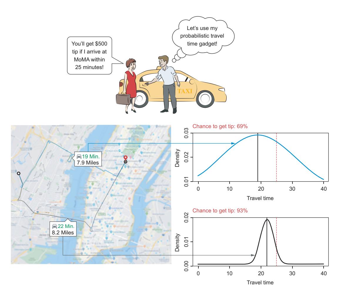
have the better chance of getting the $500 tip? To answer this question, you can look at the distributions on the right side of figure 1.1. After a quick eyeball analysis, you conclude that you have a better chance of getting the tip when taking the lower route, even though it has a larger mean travel time. The reason is that the narrow distribution of the lower route has a larger fraction of the distribution corresponding to travel times shorter than 25 minutes. To support your assessment with hard numbers, you can use the satnav tool with the probabilistic model to compute for both distributions the probability of arriving at MoMA in less than 25 minutes. This probability corresponds to the proportion of the area under the curve left of the dashed line in figure 1.1, which indicates a critical value of 25 minutes. Letting the tool compute the probabilities from the distribution, you know that your chance of getting the tip is 93% when taking the lower route and only 69% when taking the upper road.

As discussed in this cab driver example, the main advantages of probabilistic models are that these can capture the uncertainties in most real-world applications and provide essential information for decision making. Other examples of the use of probabilistic models include self-driving cars or digital medicine probabilistic models. You can also use probabilistic DL to generate new data that is similar to your observed data. A famous fun application is to create realistic looking faces of non-existing people. We talk about this in chapter 6. Let’s first look at DL from a bird’s-eye view before peeking into the curve-fitting part.

1.2 A first brief look at deep learning (DL)

What is DL anyway? When asked for a short elevator pitch, we would say that it’s a machine learning (ML) technique based on artificial neural networks (NNs) and that it’s loosely inspired by the way the human brain works. Before giving our personal definition of DL, we first want to give you an idea of what an artificial NN looks like (see figure 1.2).

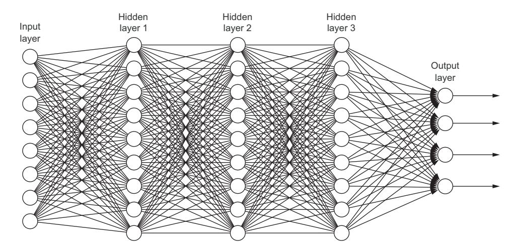
Figure 1.2 An example of an artificial neural network (NN) model with three hidden layers. The input layers hold as many neurons as we have numbers to describe the input.

In figure 1.2, you can see a typical traditional artificial NN with three hidden layers and several neurons in each layer. Each neuron within a layer is connected with each neuron in the next layer.

An artificial NN is inspired by the brain that consists of up to billions of neurons processing, for example, all sensory perceptions such as vision or hearing. Neurons within the brain aren’t connected to every other neuron, and a signal is processed through a hierarchical network of neurons. You can see a similar hierarchical network structure in the artificial NN shown in figure 1.2. While a biological neuron is quite complex in how it processes information, a neuron in an artificial NN is a simplification and abstraction of its biological counterpart.

To get a first idea about an artificial NN, you can better imagine a neuron as a container for a number. The neurons in the input layer are correspondingly holding the numbers of the input data. Such input data could, for example, be the age (in years), income (in dollars), and height (in inches) of a customer. All neurons in the following layers get the weighted sum of the values from the connected neurons in the previous layer as their input. In general, the different connections aren’t equally important but have weights, which determine the influence of the incoming neuron’s value on the neuron’s value in the next layer. (Here we omit that this input is further transformed within the neuron.) DL models are NNs, but they also have a large number of hidden layers (not just three as in the example from figure 1.2).

The weights (strength of connections between neurons) in an artificial NN need to be learned for the task at hand. For that learning step, you use training data and tune the weights to optimally fit the data. This step is called fitting. Only after the fitting step can you use the model to do predictions on new data.

Setting up a DL system is always a two-stage process. In the first step, you choose an architecture. In figure 1.2, we chose a network with three layers in which each neuron from a given layer is connected to each neuron in the next layer. Other types of networks have different connections, but the principle stays the same. In the next step, you tune the weights of the model so that the training data is best described. This fitting step is usually done using a procedure called gradient descent. You’ll learn more about gradient descent in chapter 3.

Note that this two-step procedure is nothing special to DL but is also present in standard statistical modeling and ML. The underlying principles of fitting are the same for DL, ML, and statistics. We’re convinced that you can profit a lot by using the knowledge that was gained in the field of statistics during the last centuries. This book acknowledges the heritage of traditional statistics and builds on it. Because of this, you can understand much of DL by looking at something as simple as linear regression, which we introduce in this chapter and use throughout the book as an easy example. You’ll see in chapter 4 that linear regression already is a probabilistic model providing more information than just one predicted output value for each sample. In that chapter, you’ll learn how to pick an appropriate distribution to model the variability of the outcome values. In chapter 5, we’ll show you how to use the TensorFlow Probability

framework to fit such a probabilistic DL model. You can then transfer this approach to new situations allowing you to design and fit appropriate probabilistic DL models that not only provide high performance predictions but also capture the noise of the data.

1.2.1 A success story

DL has revolutionized areas that so far have been especially hard to master with traditional ML approaches but that are easy to solve by humans, such as the ability to recognize objects in images (computer vision) and to process written text (natural language processing) or, more generally, any kind of perception tasks. Image classification is far from being only an academic problem and is used for a variety of applications:

• Face recognition
• Diagnostics of brain tumors in MRI data
• Recognition of road signs for self-driving cars

Although DL reveals its potential in different application areas, probably the easiest to grasp is in the field of computer vision. We therefore use computer vision to motivate DL by one of its biggest success stories.

In 2012, DL made a splash when Alex Krizhevsky from Geoffrey Hinton’s lab crushed all competitors in the internationally renowned ImageNet competition with a DL-based model. In this competition, teams from leading computer vision labs trained their models on a big data set of ~1 million images with the goal of teaching these to distinguish 1,000 different classes of image content. Examples for such classes are ships, mushrooms, and leopards. In the competition, all trained models had to list the five most probable classes for a set of new test images. If the right class wasn’t among the proposed classes, the test image counted as an error (see figure 1.3, which shows how DL-based approaches took image classification by storm).

Before DL entered the competition, the best programs had an error rate of ~25%. In 2012, Krizhevsky was the first to use DL and achieved a huge drop in the error rate (by 10% to only ~15%). Only a year later, in 2013, almost all competitors used DL, and in 2015, different DL-based models reached the level of human performance, which is about 5%. You might wonder why humans misclassify 1 image in 20 (5%). A fun fact: there are 170 different dog breeds in that data set, which makes it a bit harder for humans to correctly classify the images.

1.3 Classification

Let’s look at the differences between non-probabilistic, probabilistic, and Bayesian probabilistic classification. DL is known to outperform traditional methods, especially in image classification tasks. Before going into details, we want to use a face recognition problem to give you a feeling for the differences and the commonalities between a DL approach and a more traditional approach to face recognition. As a side note, face recognition is actually the application that initially brought us into contact with DL.

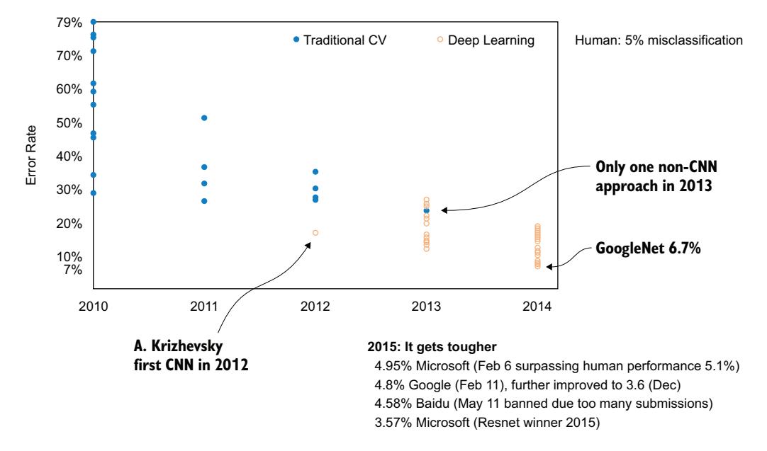
Figure 1.3 The impressive results of DL in the ImageNet competition

As statisticians, we had a collaboration project with some computer science colleagues for doing face recognition on a Raspberry Pi minicomputer. The computer scientists challenged us by kidding about the age of the used statistical methods. We took the challenge and brought them to a surprised silence by proposing DL to tackle our face recognition problem. The success in this first project triggered many other joint DL projects, and our interests grew, looking deeper into the underlying principles of these models.

Let’s look at a specific task. Sara and Chantal were together on holidays and took many pictures, each showing at least one of them. The task is to create a program that can look at a photo and determine which of the two women is in the photo. To get a training data set, we labeled 900 pictures, 450 for each woman, with the name of the pictured woman. You can imagine that images can be very different at first sight because the women might be pictured from different angles, laughing or tired, dressed up or casual, or having a bad hair day. Still, for you, the task is quite easy. But for a computer, an image is only an array of pixel values, and programming it to tell the difference between two women is far from trivial.

1.3.1 Traditional approach to image classification

A traditional approach to image classification doesn’t directly start with the pixel values of the images but tackles the classification task in a two-step process. As a first step, experts in the field define features that are useful to classify the images. A simple example of such a feature would be the mean intensity value of all pixels, which can

be useful to distinguish night shots from pictures taken during the day. Usually these features are more complex and tailored to a specific task. In the face recognition problem, you can think about easily understandable features like the length of the nose, width of the mouth, or the distance between the eyes (figure 1.4).

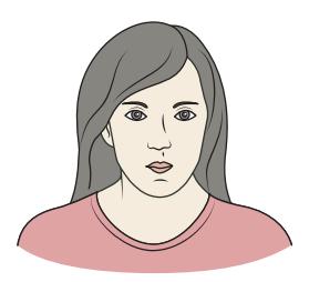
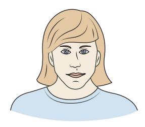
Figure 1.4 Chantal (left) has a large distance between the eyes and a rather small mouth. Sara (right) has a small distance between the eyes and a rather large mouth.

But these kinds of high-level features often are difficult to determine because many aspects need to be taken into account, such as mimics, scale, receptive angle, or light conditions. Therefore, non-DL approaches often use less interpretable, low-level features like SIFT features (Scale-Invariant Feature Transform), capturing local image properties such as magnification or rotation that are invariant to transformations. You can, for example, think about an edge detector: an edge won’t disappear if the image is rotated or scaled.

Already this simple example makes clear that feature engineering, meaning defining and extracting those properties from the image that are important for the classification, is a complicated and time-consuming task. It usually requires a high level of expertise. The (slow) progress in many applications of computer vision like face recognition was mainly driven by the construction of new and better features.

NOTE You need to extract all these features from all images before you can tackle the actual classification task.

After the features-extraction step, the values of these features represent each image. In order to identify Sara or Chantal from this feature representation of the image, you need to choose and fit a classification.

What is the task of such a classification model? It should discriminate between the different class labels. To visualize this idea, let’s imagine that an image is described by only two features: say, distance of the eyes and width of the mouth. (We are aware that in most real cases, a good characterization of an image requires many more features.)

Because the women aren’t always pictured head on but from different viewpoints, the apparent distance between the eyes isn’t always the same for the same women. The apparent width of the mouth can vary even more, depending if the woman laughs or makes an air-kiss. When representing each image of the pictured woman by these two features, the feature space can be visualized by a 2D plot. One axis indicates the eye distance and the other axis shows the mouth width (see figure 1.5). Each image is represented by a point; images of Sara are labeled with an S and images of Chantal with a C.

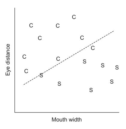
Figure 1.5 A 2D space spanned by the features mouth width and eye distance. Each point represents an image described by these two features (S for Sara and C for Chantal). The dashed line is a decision boundary separating the two classes.

One way you can think about a non-probabilistic classification model is that the model defines decision boundaries (see the dashed line in figure 1.5) that split the feature space into different regions. Each resulting region corresponds to one class label. In our example, we’ve determined a Sara region and a Chantal region. You can now use this decision boundary to classify new images from which you only know the values for the two features: if the corresponding point in the 2D feature space ends up in the Sara region, you classify it as Sara; otherwise, as Chantal.

You might know from your data analysis experiences some methods like the following, which you can use for classification. (Don’t worry if you aren’t familiar with these methods.)

• Logistic or multinomial regression
• Random forest
• Support vector machines
• Linear discriminant analysis

Most classification models, including the listed methods and also DL, are parametric models, meaning the model has some parameters that determine the course of the boundaries. The model is only ready to actually perform a classification or class probability prediction after replacing the parameters by certain numbers. Fitting is about how to find these numbers and how to quantify the certainty of these numbers.

Fitting the model to a set of training data with known class labels determines the values of the parameter and fixes the decision boundaries in the feature space. Depending on the classification method and the number of parameters, these decision boundaries could be simple straight lines or a complex boundary with wiggles. You can summarize the traditional workflow to set up a classification method in three steps:

• ¹ Defining and extracting features from the raw data
• ² Choosing a parametric model
• ³ Fitting the classification model to the data by tuning its parameter

To evaluate the performance of the models, you use a validation data set that is not used during the training. A validation data set in the face recognition example would consist of new images of Chantal and Sara that were not part of the training data set. You then can use the trained model to predict the class label and use the percentage of correct classifications as a (non-probabilistic) performance measure.

Depending on the situation, one or another classification method will achieve better results on the validation data set. However, in classical image classification, the most important ingredient for success isn’t the choice of the classification algorithm but the quality of the extracted image features. If the extracted features take different values for images from different classes, you’ll see a clear separation of the respective points in the feature space. In such a situation, many classification models show a high classification performance.

With the example of discriminating Sara from Chantal, you went through the traditional image classification workflow. For getting good features, you first had to recognize that these two women differ in their mouth width and their eye distance. With these specific features, you saw that it is easy to build a good classifier. However, for discriminating between two other women, these features might not do the trick, and you would need to start over with the feature developing process again. This is a common drawback when working with customized features.

1.3.2 Deep learning approach to image classification

In contrast to the traditional approach to image classification, the DL approach starts directly from the raw image data and uses only the pixel values as the input features to the model. In this feature representation of an image, the numbers of pixels define the dimension of the feature space. For a low-resolution picture with 100 × 100 pixels, this already amounts to 10,000.

Besides such a high dimension, the main challenge is that pixel similarity of two pictures doesn’t imply that the two images correspond to the same class label. Figure 1.6 illustrates where the images in the same column obviously correspond to the same class but are different on the pixel level. Simultaneously, images in the same row of figure 1.6 show high pixel similarity but don’t correspond to the same class.

The core idea of DL is to replace the challenging and time-consuming task of feature engineering by incorporating the construction of appropriate features into the fitting process. Also, DL can’t do any magic so, similar to traditional image analysis, the features have to be constructed from the pixel values at hand. This is done via the hidden layers of the DL model.

Each neuron combines its inputs to yield a new value, and in this manner, each layer yields a new feature representation of the input. Using many hidden layers allows the NN to decompose a complicated transformation from the raw data to the outcome in a hierarchy of simple transformations. When going from layer to layer, you get a more and more abstract representation of the image that becomes better suited for discriminating between the classes. You’ll learn more about this in chapter 2, where you’ll see that during the fitting process of a DL model, a hierarchy of successively more complex features is learned. This then allows you to discriminate between the different classes without the need of manually specifying the appropriate features.

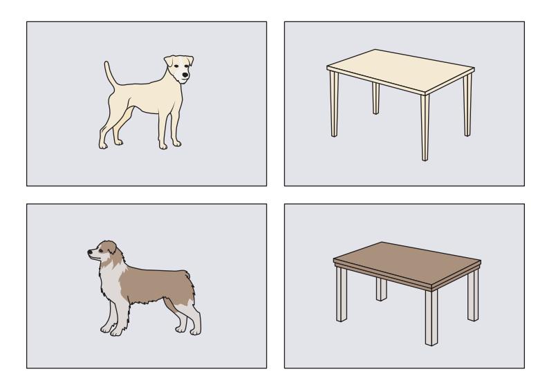
Figure 1.6 The left column shows two images of the class dog. The right column shows two images of the class table. When comparing the pictures on the pixel level, the two images in the same column are less similar than the two images in the same row, even if one image in a row shows a dog and the other image displays a table.

Branding DL (deep learning)

In the earlier days of machine learning (ML), neural networks (NNs) were already around, but it was technically impossible to train deep NNs with many layers, mainly because of a lack of computer power and training data. With the technical obstacles resolved, some tricks have been discovered that made it possible to train NNs with several hundred layers.

Why do we talk about DL instead of artificial NNs? DL sells better than artificial NNs. This might sound disrespectful, but such rebranding was probably a smart move, especially because NNs haven’t delivered what was promised during the last decades and, therefore, gained a somewhat bad reputation. We work with “deep” NNs with many hidden layers. This leads to a deep hierarchy in the construction of features, allowing these to become more abstract with every step up in the hierarchy.

After defining the architectures, the network can be understood as a parametric model that often contains millions of parameters. The model takes an input x and produces an output y. This is true for every DL model (including reinforcement learning). The DL modeling workflow can be summarized in two steps:

• ¹ Defining the DL model architecture
• ² Fitting the DL model to the raw data

The next sections discuss what is meant by non-probabilistic and probabilistic classification models and what benefits you can get from a Bayesian variant of a probabilistic classification model.

1.3.3 Non-probabilistic classification

Let’s first look at non-probabilistic classification. To make it easy and illustrative, we use the image classification example again. The goal in image classification is to predict for a given image which class it corresponds to. In the ImageNet competition in section 1.2, there were 1,000 different classes. In the face recognition example, there were only two classes: Chantal and Sara.

In non-probabilistic image classification, you only get the predicted class label for each image. More precisely, a non-probabilistic image classifier takes an image as input and then predicts only the best guess for the class as output. In the face recognition example, it would either output Chantal or Sara. You can also think about a non-probabilistic model as a deterministic model without any uncertainty. When looking with probabilistic glasses at a non-probabilistic model, it seems that a non-probabilistic model is always certain. The non-probabilistic model predicts with a probability of one that the image belongs to one specific class.

Imagine a situation where the image shows Chantal where she dyes her hair the same color as that of Sara and the hair covers Chantal’s face. For a human being, it’s quite hard to tell if the image shows Chantal or Sara. But the non-probabilistic classifier still provides a predicted class label (for example, Sara) without indicating any uncertainty. Or imagine an even more extreme situation where you provide an image that shows neither Chantal nor Sara (see figure 1.7). Which prediction will you get from the classifier? You would like the classifier to tell you that it is not able to make a reliable prediction. But a non-probabilistic classifier still yields either Chantal or Sara as a prediction without giving a hint of any uncertainty. To tackle such challenges of handling difficult or novel situations, we turn to probabilistic models and their Bayesian variants. These can express their uncertainty and indicate potentially unreliable predictions.

1.3.4 Probabilistic classification

The special thing in probabilistic classification is that you not only get the best guess for the class label but also a measure for the uncertainty of the classification. The uncertainty is expressed by a probability distribution. In the face recognition example, a probabilistic classifier would take a face image and then output a certain probability for Chantal and for Sara. Both probabilities add up to 1 (see figure 1.8).

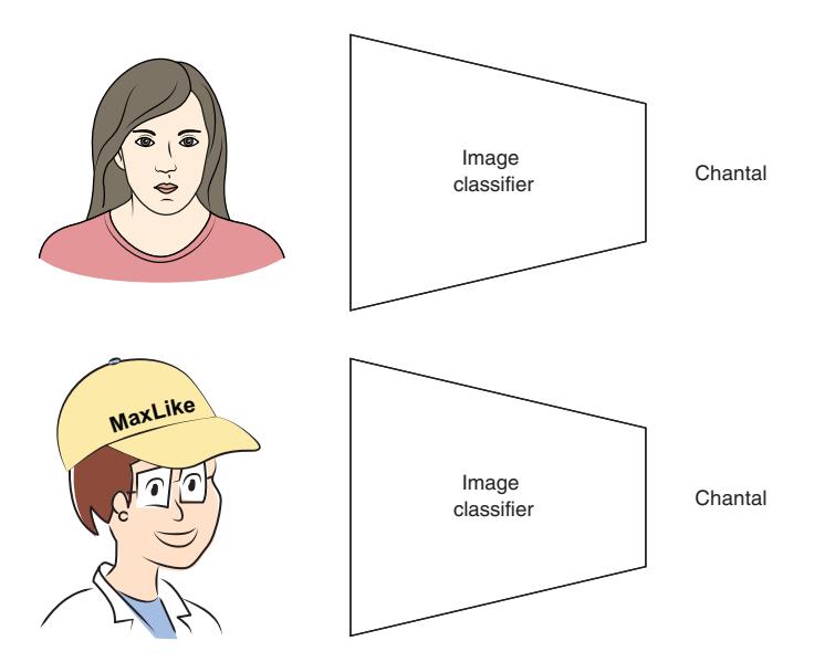
Figure 1.7 A non-probabilistic image classifier for face recognition takes as input an image and yields as outcome a class label. Here the predicted class label is Chantal, but only the upper image really shows Chantal. The lower image shows a woman who is neither Chantal nor Sara.

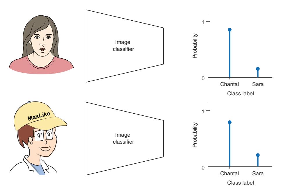
Figure 1.8 A probabilistic image classifier for face recognition takes as input an image and yields as outcome a probability for each class label. In the upper panel, the image shows Chantal, and the classifier predicts a probability of 0.85 for the class Chantal and a probability of 0.15 for the class Sara. In the lower panel, the image shows neither Chantal nor Sara, and the classifier predicts a probability of 0.8 for the class Chantal and a probability of 0.2 for the class Sara.

To give a best single guess, you would pick the class with the highest probability. It is common to think about the probability of the predicted class as an uncertainty of the prediction. This is the case when all the images are sufficiently similar to the training data.

But in reality, this is not always the case. Imagine that you provide the classifier with an image that shows neither Chantal nor Sara. The classifier has no other choice than to assign probabilities to the classes Chantal or Sara. But you would hope that the classifier shows its uncertainty by assigning more or less equal probabilities to the two possible but wrong classes. Unfortunately, this is often not the case when working with probabilistic NN models. Instead, often quite high probabilities are still assigned to one of the possible but wrong classes (see figure 1.8). To tackle this problem, in part 3 of our book, we extend the probabilistic models by taking a Bayesian approach, which can add an additional uncertainty that you can use to detect novel classes.

1.3.5 Bayesian probabilistic classification

The nice thing about Bayesian models is that these can express uncertainty about their predictions. In our face recognition example, the non-Bayesian probabilistic model predicts an outcome distribution that consists of the probability for Chantal and the probability for Sara, which add up to 1. But how certain is the model about the assigned probabilities? Bayesian models can give an answer to this question. In part 3 of this book, you will learn how this is done in detail. At this point, let’s just note that you can ask a Bayesian model several times and get different answers when you ask it. This reflects the uncertainty inherent in the model (see figure 1.9). Don’t worry if you do not see how you get these different model outputs for the same input. You will learn about that in the third part of the book.

The main advantage of Bayesian models is that these can indicate a non-reliable prediction by a large spread of the different sets of predictions (see lower panel of figure 1.9). In this way, you have a better chance to identify novel classes like the young lady in the lower panel of figure 1.9 who is neither Chantal nor Sara.

1.4 Curve fitting

We want to finish this introductory chapter talking about the differences in probabilistic and non-probabilistic DL methods on regression tasks. Regression is sometimes also referred to as curve fitting. This reminds one of the following:

All the impressive achievements of deep learning amount to just curve fitting.

—Judea Pearl, 2018

When we heard that Judea Pearl, the winner of the prestigious Turing Award in 2011 (the computer science equivalent of the Nobel prize), claimed DL to be just curve fitting (the same curve fitting done in simple analysis like linear regression for centuries), at first we were surprised and even felt a bit offended. How could he be so

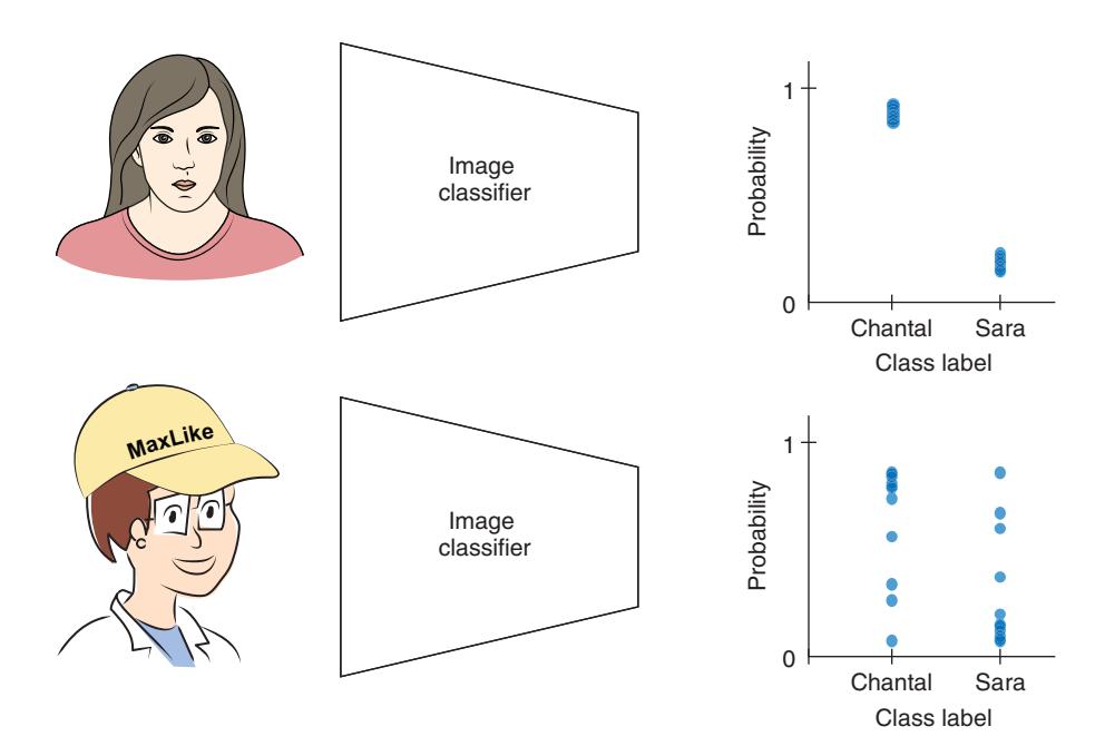
Figure 1.9 A Bayesian probabilistic image classifier for face recognition takes as input an image and yields as outcome a distribution of probability sets for the two class labels. In the upper panel, the image is showing Chantal, and the predicted sets of probabilities all predict a large probability for Chantal and an accordingly low probability for Sara. In the lower panel, the image shows a lady who is neither Chantal nor Sara, so the classifier predicts different sets of probabilities indicating a high uncertainty.

disrespectful about our research subject, which, moreover, showed such impressive results in practice? Our relative calmness is probably due to the fact that we aren’t computer scientists but have a background in physics and statistical data analysis. Curve fitting isn’t just curve fitting for us. However, giving his statement a second thought, we can see his point: the underlying principles of DL and curve fitting are identical in many respects.

1.4.1 Non-probabilistic curve fitting

Let’s first take a closer look at the non-probabilistic aspects of traditional curve-fitting methods. Loosely speaking, non-probabilistic curve fitting is the science of putting lines through data points. With linear regression in its most simple form, you put a straight line through the data points (see figure 1.10). In that figure, we assume that we have only one feature, x, to predict a continuous variable, y. In this simple case, the linear regression model has only two parameters, a and b :

$$u = a cdot x + b$$

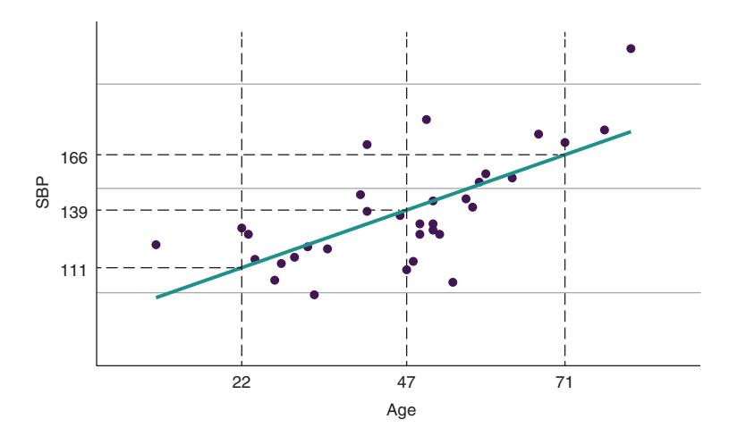
Figure 1.10 Scatter plot and regression model for the systolic blood pressure (SBP) example. The dots are the measured data points; the straight line is the linear model. For three age values (22, 47, 71), the positions of the horizontal lines indicate the predicted best guesses for the SBP (11, 139, 166).

After the definition of the model, the parameters a and b need to be determined so that the model can be actually used to predict a single best guess for the value of y when given x. In the context of ML and DL, this step of finding good parameter values is called training. But how are networks trained? The training of the simple linear regression and DL models is done by fitting the model’s parameters to the training data—a.k.a. curve fitting.

Note that the number of parameters can be vastly different, ranging from 2 in the 1D linear regression case to 500 million for advanced DL models. The whole procedure is the same as in linear regression. You’ll learn in chapter 3 how to fit the parameter of a non-probabilistic linear regression model.

So, what do we mean when we say a non-probabilistic model is fit to data? Let’s look at the model for a concrete example of predicting the blood pressure y based on the age x. Figure 1.10 is a plot of the systolic blood pressure (SBP) against the age for 33 American women. Figure 1.10 shows concrete realizations with a = 1.70 and b = 87.7 (the solid line). In a non-probabilistic model, for each age value you get only one best guess for the SBP for women of this age. In figure 1.10, this is demonstrated for three age values (22, 47, and 71), where the predicted best guesses for the SBP (111, 139, and 166) are indicated by the positions of the dashed horizontal lines.

1.4.2 Probabilistic curve fitting

What do you get when you fit a probabilistic model to the same data? Instead of only a single best guess for the blood pressure, you get a whole probability distribution. This tells you that women with the same age might well have different SBPs (see figure 1.11).

In the non-probabilistic linear regression, an SBP of 111 is predicted for 22-year-old women (see figure 1.10). Now, when looking at the predicted distribution for 22 year-old women, SBP values close to 111 (the peak of the distribution) are expected with higher probability than values further away from 111.

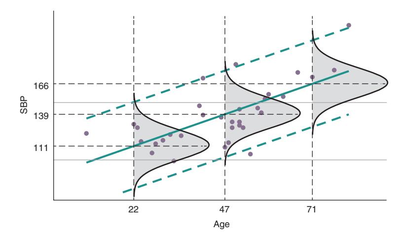
Figure 1.11 Scatter plot and regression model for the systolic blood pressure (SBP) example. The dots are the measured data points. At each age value (22, 47, 71), a Gaussian distribution is fitted that describes the probability distribution of possible SBP values of women in these age groups. For the three age values, the predicted probability distributions are shown. The solid line indicates the positions of the mean values of all distributions corresponding to the ages between 16 and 90 years. The upper and lower dashed lines indicate an interval in which 95% of all values are expected by the model.

The solid line in figure 1.10 indicates the positions of the mean values of all distributions corresponding to the age values between 16 and 90 years. The solid line in figure 1.11 exactly matches the regression line in figure 1.10, which is predicted from a non-probabilistic model. The dashed lines that are parallel to the mean indicate an interval in which 95% of all individual SBP values are expected by the model.

How do you find the optimal values for the parameters in a non-probabilistic and a probabilistic model? Technically, you use a loss function that describes how poorly the model fits the (training) data and then minimizes it by tuning the weights of the model. You’ll learn about loss functions and how to use these for fitting non-probabilistic or probabilistic models in chapters 3, 4, and 5. You’ll then see the difference between the loss function of a non-probabilistic and a probabilistic model.

The discussed linear regression model is, of course, simple. We use it mainly to explain the underlying principles that stay the same when turning to complex DL models. In real world applications, you would often not assume a linear dependency,

and you would also not always want to assume that the variation of the data stays constant. You’ll see in chapter 2 that it’s easy to set up a NN that can model non-linear relationships. In chapters 4 and 5, you’ll see that it is also not hard to build a probabilistic model for regression tasks that can model data with non-linear behavior and changing variations (see figure 1.12). To evaluate the performance of a trained regression model, you should always use a validation data set that is not used during training. In figure 1.12, you can see the predictions of a probabilistic DL model on a new validation set that shows that the model is able to capture the non-linear behavior of the data and also the changing data variation.

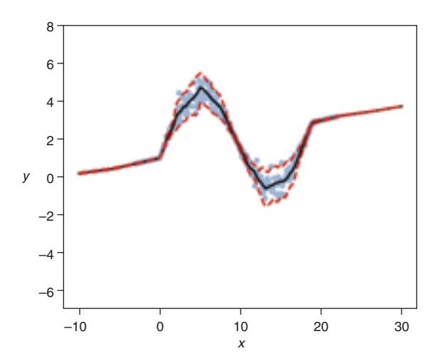
Figure 1.12 Scatter plot and validation data predictions from a (non-Bayesian) probabilistic regression model. The model is fitted on some simulated data with a non-linear dependency between x and y and with non-constant data variation. The solid line indicates the positions of the mean values of all predicted distributions. The upper and lower dashed lines indicate an interval in which 95% of all values are expected by the model.

What happens if we use the model to predict the outcome of x values outside the range of the training data? You can get a first glimpse when looking at figure 1.12, where we only have data between –5 and 25 but show the predictions in a wider range between –10 and 30. It seems that the model is especially certain about its predictions in the ranges where it has never seen the data. That is strange and not a desirable property of a model! The reason for the model’s shortcoming is that it only captures the data variation—it does not capture the uncertainty about the fitted parameters. In statistics, there are different approaches known to capture this uncertainty; the Bayesian approach is among these. When working with DL models, the Bayesian approach is the most feasible and appropriate. You will learn about that in the last two chapters of this book.

1.4.3 Bayesian probabilistic curve fitting

The main selling point of a Bayesian DL model is its potential to sound the alarm in case of novel situations for which the model was not trained. For a regression model, this corresponds to extrapolation, meaning you use your model in a data range that is

outside the range of the training data. In figure 1.13, you can see the result of a Bayesian variant of the NN that produces the fit shown in figure 1.12. It is striking that only the Bayesian variant of the NN raises the uncertainty when leaving the range of the training data. This is a nice property because it can indicate that your model might yield unreliable predictions.

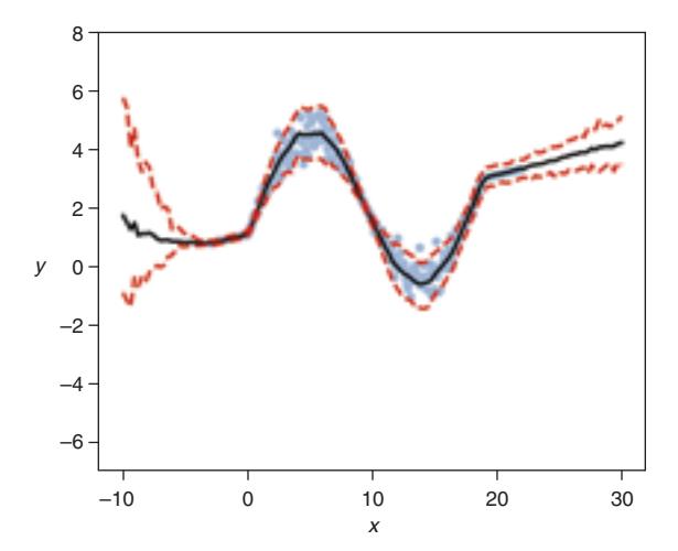
Figure 1.13 Scatter plot and validation data predictions from a Bayesian probabilistic regression model. The model was fitted on some simulated data with non-linear dependency between x and y and nonconstant data variation. The solid line indicates the positions of the mean values of all predicted distributions. The upper and lower dashed lines indicate an interval in which 95% of all values are expected by the model.

1.5 When to use and when not to use DL?

Recently, DL has had several extraordinary success stories. You therefore might ask yourself whether you should forget about traditional ML approaches and use DL instead. The answer depends on the situation and the task at hand. In this section, we cover when not to use DL as well as what problems DL is useful for.

1.5.1 When not to use DL

DL typically has millions of parameters and, therefore, usually needs a lot of data to be trained. If you only have access to a limited number of features that describe each instance, then DL isn’t the way to go. This includes the following applications:

• Predict the scores of a student in their first university year based on only their scores in high school
• Predict the risk for a heart attack within the next year based on the sex, age, BMI (body mass index), blood pressure, and blood cholesterol concentration of a person
• Classify the sex of a turtle based on its weight, its height, and the length of its feet

Also, in situations where you have only few training data and you know exactly which features determine the outcome of interest (and it’s easy for you to extract these features from your raw data), then you should go for these features and use those as a basis for a traditional ML model. Imagine, for example, you get images from a soccer
player collection of different individual French and Dutch soccer players. You know that the jerseys of the French team are always blue, and those of the Dutch team are always orange. If your task is to develop a classifier that discriminates between players of these two teams, it’s probably best to decide if the number of blue pixels (the French team) in the image is larger than the number of orange pixels (the Dutch team). All other features (such as hair color, for example) that seem to discriminate between the two teams would add noise rather than help with the classification of new images. It’s therefore probably not a good idea to extract and use additional features for your classifier.

1.5.2 When to use DL

DL is the method of choice in situations where each instance is described by complex raw data (like images, text, or sound) and where it isn’t easy to formulate the critical features that characterize the different classes. DL models are then able to extract features from the raw data that often outperform models that rely on handcrafted features. Figure 1.14 displays various tasks in which DL recently changed the game.

	Input x to DL model	Output y of DL model	Application
Type	Example	Type	Example
Images		Label	“Tiger”	Image classification
Audio		Sequence/Text	“See you tomorrow.”	Voice recognition
ASCII sequences	“Hallo, wie gehts?”	Unicode sequences		Translation
Environment	The input is twofold. The first is the state of the world.The second part of the input is the reward for the last action (whether it was good or bad).	The output of the neural network is an action the agent does next.	Walk left/place stone at certain position on the Go board	Deep reinforcement learning; for example, Go

Figure 1.14 The various tasks recently solved by DL that were out-of-reach for traditional ML for a long time

1.5.3 When to use and when not to use probabilistic models?

You will see in this book that for most DL models, it is possible to set up a probabilistic version of the model. You get the probabilistic version basically for free. In these cases, you can only gain when using the probabilistic variant because it provides not only the
information that you get from the non-probabilistic version of the model, but also additional information that can be essential for decision making. If you use a Bayesian variant of a probabilistic model, you have the additional advantage of getting a measure that includes the model’s parameter uncertainty. Having an uncertainty measure is especially important to identify situations in which your model might yield unreliable predictions.

1.6 What you’ll learn in this book

This book gives you a hands-on introduction to probabilistic DL. We’ll provide exercises and code demos as Jupyter notebooks, which allow you to get experiences and so gain a deeper understanding of the concepts. To benefit from this book, you should already know how to run simple Python programs and how to fit a model to data (a simple model such as a linear regression is fine). For a deep understanding of the more advanced sections (indicated by an asterisk after the end of the heading), you should be fluent with intermediate math such as matrix algebra and differential calculus, as well as with intermediate statistics such as interpreting probability distributions. You will learn how to

• Implement DL models with different architectures by using the Keras framework
• Implement a probabilistic DL model, predicting from a given input a whole distribution for the outcome
• For a given task, choose an appropriate outcome distribution and loss function by using the maximum likelihood principle and the TensorFlow Probability framework
• Set up flexible probabilistic DL models such as currently used state-of-the-art models for image generation of text to speech translations
• Build Bayesian variants of DL models that can express uncertainties, letting you identify non-reliable predictions

We’ll introduce you to the different DL architectures in the next chapter.

Summary

• Machine learning (ML) methods were invented to allow a computer to learn from data.
• Artificial neural networks (NNs) are ML methods that start from raw data and include the feature extraction process as part of the model.
• Deep learning (DL) methods are NNs that are called deep because they have a large number of layers.
• DL outperforms traditional ML methods in perceptual tasks such as grasping the content of an image or translating text to speech.
• Curve fitting is a technique that fits a model (the curve or a distribution) to data.
• DL and curve fitting are similar and rely on the same principles. These principles are at the heart of this book. Understanding these lets you build better-performing DL models in terms of accuracy, calibration, and the ability to quantify uncertainty measures for the predictions.
• Probabilistic models go beyond single value predictions and capture the variation of real data and the uncertainty of the model fit, which allows for better decision making.
• Bayesian variants of probabilistic models can help to identify unreliable predictions.

Neural network architectures

This chapter covers

• Needing different network types for different data types
• Using fully connected neural networks for tabular-like data
• Using 2D convolutional neural networks for image-like data
• Using 1D convolutional neural networks for ordered data

The vast majority of DL models are based on one or a combination of three types of layers: fully connected, convolutional, and recurrent. The success of a DL model depends in great part on choosing the right architecture for the problem at hand.
If you want to analyze data that has no structure, like tabular data in Excel sheets, then you should consider fully connected networks. If the data has a special local structure like images, then convolutional neural networks (NNs) are your friends. Finally, if the data is sequential like text, then the easiest option is to use 1D convolutional networks. This chapter gives you an overview of the different architectures used in DL and provides hints as to when to use which architectural type.

2.1 Fully connected neural networks (fcNNs)

Before diving into the details of the different DL architectures, let’s look at figure 2.1. Recall the architecture of a typical traditional artificial NN that we discussed in chapter 1. The visualized NN has three hidden layers, each holding nine neurons. Each neuron within a layer connects with each neuron in the next layer. This is why this architecture is called a densely connected NN or a fully connected neural network (fcNN).

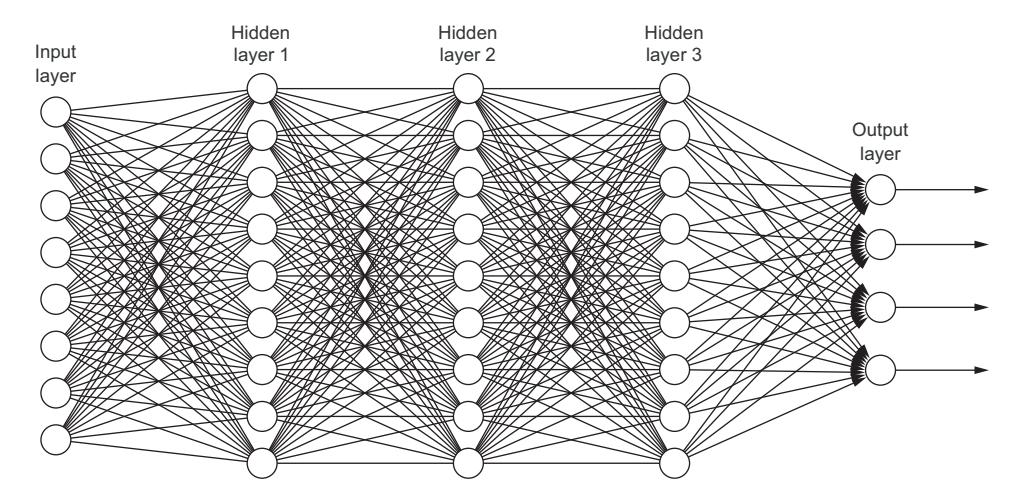
model with three hidden layers”)

Figure 2.1 An example of a fully connected neural network (fcNN) model with three hidden layers

2.1.1 The biology that inspired the design of artificial NNs

The design of NNs is inspired by the way the brain works. You shouldn’t overstretch this point; it’s just a loose inspiration. The brain is a network of neurons. The human brain has about 100 billion neurons, and each neuron, on average, connects with 10,000 other neurons. Let’s take a look at the brain’s basic unit—the neuron (see figure 2.2).

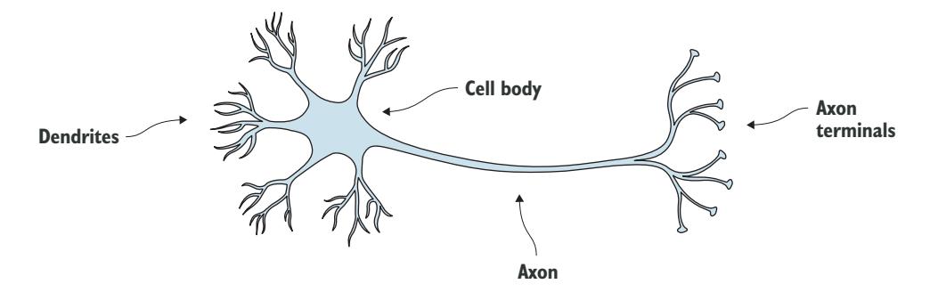
Figure 2.2 A single biological brain cell. The neuron receives the signal from other neurons via its dendrites (shown on the left). If the accumulated signal exceeds a certain value, an impulse is sent via the axon to the axon terminals (on the right), which, in turn, couple to other neurons.

Figure 2.2 shows a very simplified sketch of a neuron. It receives signals from other neurons via its dendrites. Some inputs have an activating impact, and some inputs have an inhibiting impact. The received signal accumulates and is processed within the cell body of the neuron. If the signal is strong enough, the neuron fires. That means it produces a signal that’s transported to the axon terminals. Each axon terminal connects to another neuron. Some connections can be stronger than others, which makes it easier to transduce the signal to the next neuron. Experiences and learning can change the strength of these connections. Computer scientists have derived a mathematical abstraction from the biological brain cell: the artificial neuron shown in figure 2.3.

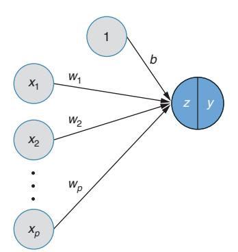
Figure 2.3 The mathematical abstraction of a brain cell (an artificial neuron). The value z is computed as the weighted sum of the input values p, x1 to xp, and a bias term b that shifts up or down the resulting weighted sum of the inputs. The value y is computed from z by applying an activation function.

An artificial neuron receives some numeric input values, xi, which are multiplied with some corresponding numeric weights, wi. To accumulate the inputs, determine the weighted sum of the inputs plus a bias term b (that gets 1 as input) as a non-linear activation function, the so-called sigmoid function, which transfers z to a number between 0 and 1 (see figure 2.4). This function is given by:

$$y = sigma(z) = frac{1}{1 + e^{-z}} = frac{e^z}{1 + e^z}$$

As you can see in figure 2.4, large positive values of z result in values close to 1, and negative values with large absolute values result in values close to 0. In this sense, the resulting value y can be interpreted as the probability that the neuron fires. Or, in the context of classification, as a probability for a certain class. If you want to build a binary classifier (with 0 and 1 as possible classes), which takes several numeric features, $x_i$, and generates the probability for class 1, then you can use a single neuron. If you have a background in statistics, this might look familiar, and indeed, a network with a single neuron is known in statistics also as logistic regression. But no need to worry if you’ve never heard of logistic regression.

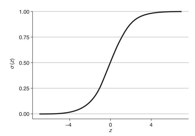
Figure 2.4 The sigmoid function f translating (squeezing) an arbitrary number z to a number between 0 and 1.

2.1.2 Getting started with implementing an NN

To get started working with DL, you need to know the basic data structures, the tensors, and the software packages manipulating those entities.

TENSORS: THE BASIC ENTITIES IN DL

Looking at figure 2.3, the mathematical abstraction of a neuron, you might ask the question, “What goes in and what comes out?” Assuming that p = 3 in figure 2.3, then you see three numbers $(x_1, x_2, text{ and } x_3)$ entering the neuron and a single number leaving the neuron. These three numbers can be treated as an array with one index. More complex neural networks can take a grayscale image, say of size $64 times 32$ as input, which can be also expressed as an array. But this time the array has two indices. The first index, i, ranges from 0 to 63 and the second, j, from 0 to 31.

Going further, say you have a color image with the colors red, green, and blue. For such an image, each pixel has x,y coordinates and three additional values. The image can be stored in an array with three indices (i, j, c). Taking it to the extreme, say you input a whole stack of 128 color images into the network. These could be stored in an array of (b, x, y, c) with b ranging from 0 to 127. Also, you can view the three weights in figure 2.3 as an array with one index, going from 0 to 2.

As it turns out, all quantities in DL can be put into arrays. In the context of DL, these arrays are called tensors, and from an abstract standpoint, all that happens in DL is the manipulation of tensors. The number of indices tensors have is the so-called dimension, order, or sometimes rank (so don’t get confused). Tensors of order 0, like the output of the neuron in figure 2.3, have no indices. Tensors with low orders also have special names:

• Tensors of order 0 are called scalars.
• Tensors of order 1 are called vectors.
• Tensors of order 2 are called matrices.

DL has gained enormous popularity with the availability of software frameworks built to manipulate tensors. In this book, we mainly use Keras (https://keras.io/) and TensorFlow (https://www.tensorflow.org/). Currently, these two frameworks are most often used by DL practitioners. TensorFlow is an open source framework developed by Google that comes with strong support for DL. Keras is a user-friendly, high-level neural networks API written in Python and capable of running on top of TensorFlow, allowing for fast prototyping.

To work through the exercises in this book, we recommend that you use the Google Colab environment (https://colab.research.google.com) as a cloud solution that runs in your browser. The most important frameworks, packages, and tools for DL are already installed, and you can immediately start coding. If you want to install a DL framework on your own computer, we recommend you follow the description given in chapter 3 of Chollet’s book at http://mng.bz/NKPN.

• To dig deeper into TensorFlow, Martin Görner’s tutorial is a good starting point: https://www.youtube.com/watch?v=vq2nnJ4g6N0.
• To learn more about Keras, we recommend the website https://keras.io/.

We use Jupyter notebooks (https://jupyter.org/) to provide you with some hands-on exercises and code examples. Jupyter notebooks offer the ability to mix Python, TensorFlow, and Keras code with text and Markdown. The notebooks are organized in cells containing either text or code. This lets you play around with the code by changing only the code in one cell. In many exercises, we provide large parts of the code, and you can experiment in individual cells with your own code. Feel free to also change the code at any location; you can’t break anything. While DL often involves huge data sets and needs enormous computing power, we distilled simple examples so that you can interactively work with the notebooks. We use the following icon to indicate the positions in the book where you should open a Jupyter notebook and work through the related code:

You can open these notebooks directly in Google Colab, where you can edit and run these in your browser. Colab is great, but you need to be online to use it. Another option (good for working offline) is to use the provided Docker container. For details on how to install Docker, see https://tensorchiefs.github.io/dl_book/. Within the Jupyter notebooks, we use the following icon to indicate where you should return to this book:

SETTING UP A FIRST NN MODEL TO IDENTIFY FAKE BANKNOTES

Let’s get started and do a first DL experiment. In this experiment, you use a single artificial neuron to discriminate real from fake banknotes.

HANDS-ON TIME Open http://mng.bz/lGd6, where you’ll find a data set describing 1,372 banknotes by two features and a class label y.

The two image features are based on wavelet analysis, a frequently used method in traditional image analysis. It’s common to store the input values and the target values in two separate tensors. The input data set contains 1,372 instances described by two features that you can organize in one 2D tensor. The first dimension usually describes the samples. This axis is referred to as axis 0. For the example, you have a 2D tensor with a shape (1372, 2). The target values are the true class labels that can be stored in a second 1D tensor with a shape (1372).

DL models typically run on graphic cards, also called graphic processing units (GPUs). These GPUs have limited memory. You therefore can’t process an entire data set at once. The data is split into smaller batches containing only a subset of the entire data set. These batches are called mini-batches, and a typical number of instances contained in a mini-batch is either 32, 64, or 128. In our banknote example, we use mini-batches with a size shape of 128.

Because the banknotes are described by only two features, you can easily see the positions of real and fake banknotes in the 2D feature space (see figure 2.5). Also, the boundary between the two classes isn’t separated by a straight line.

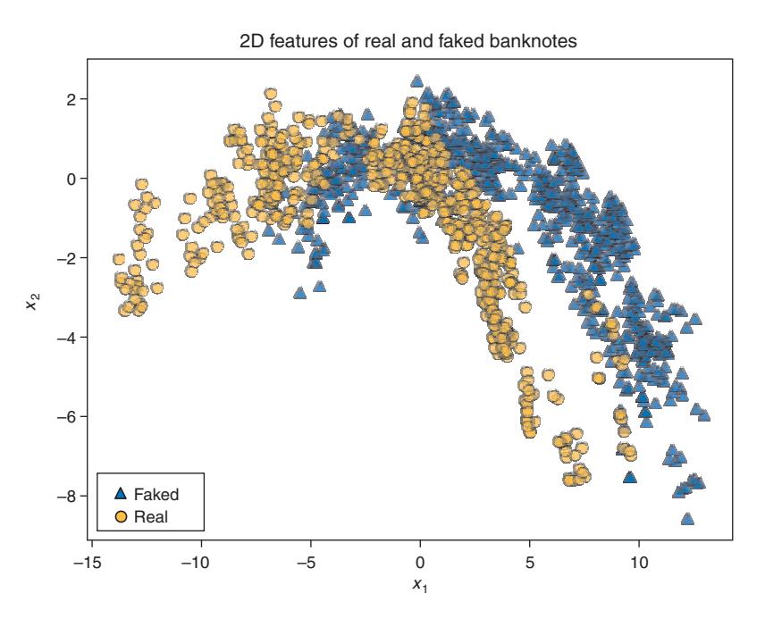
Figure 2.5 The (training) data points for the real and fake banknotes

Let’s use a single neuron with a sigmoid activation function (also known as logistic regression) as a classification model (see figure 2.6). We’ll separate the fake banknotes from the real banknotes for the data shown in figure 2.5.

Before we define the Keras code, let’s think of the tensor structure needed. What goes into the network? If you use a single training data point, it’s a vector with two entries (the next section discusses how the bias is handled). If you take a batch of size 128 of those vectors, you have a tensor of order 2 (a matrix) with the shape (128, 2). Usually one doesn’t specify the batch size when defining the network. In that case, you use None as the batch size. As in figure 2.6, the input is processed by a single neuron with sigmoid activation.

NOTE Here we only briefly discuss the main building blocks needed for our DL experiment. To learn about Keras, refer to the Keras website at https://keras.io/, and the book, Deep Learning With Python, written by the creator of Keras, François Chollet.

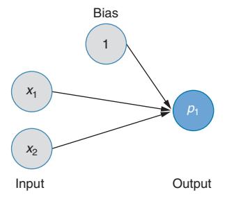
Figure 2.6 An fcNN with one single neuron. The two nodes in the input layer correspond to the two features describing each banknote. The output layer has one node that corresponds to the probability of class 1 (a fake banknote).

In listing 2.1, we use the sequential mode to define the NN model. In the sequential model definition, the layers are added one after the other. The output of one layer is the input to the next layer and so on; therefore, you usually don’t need to specify the shape of the inputs to a layer. The first layer is an exception, and here you need to specify the shape of the input.

Under the hood, Keras translates the model into tensor operations. In our simple model in listing 2.1, the dense layer, Dense(1), takes the input tensor X with the dimension (batch_size, 2), multiplies it with a 2 × 2 matrix W, and adds a bias term b. This gives a vector of length batch_size. If this sounds strange to you, take a look at chapter 2 of Chollet’s book, Deep Learning with Python, at http://mng.bz/EdPo to learn more about matrix multiplication.

After defining the model, it’s compiled, and the used loss and an optimization function need to be specified. Here we use the loss function crossentropy, which is commonly used for classification and which quantifies how well the correct class is predicted. You’ll learn more about loss functions in chapter 4. Last but not least, we optimize the weights of the model by an iterative training process, which is called stochastic gradient descent (SGD), discussed in chapter 3. The goal of the fitting process is to adapt the model weights so that the loss is minimized. The model weights are updated after each mini-batch, here containing 128 instances. One iteration over the complete training set is called an epoch; here we train for 400 epochs.

Listing 2.1 Definition of an NN with only one neuron after the input

model = Sequential()
model.add( Dense(1,
    batch_input_shape=(None, 2),
    activation='sigmoid')
)
sgd = optimizers.SGD(lr=0.15)
model.compile(
    loss='binary_crossentropy',
    optimizer=sgd
)
history = model.fit(X, Y, epochs=400,
    batch_size=128)

Sequential starts the definition of the network.
Adds a new layer to the network with a single neuron; hence, 1 in Dense(1).
The input is a tensor of size (Batch Size, 2). Using None, we don’t need to specify the batch size now.
Chooses the activation function sigmoid as in figure 2.4.
Compiles the model, which ends the definition of the model.
Defines and uses the stochastic gradient descent optimizer.
Trains the model using the data stored in X and Y for 400 epochs. Fixes the batch size to 128 examples.

{alt=”Screenshot related to the hands-on time section for the banknote notebook.”}

HANDS-ON TIME When running the code in the notebook (http://mng.bz/lGd6), you’ll observe a decreasing loss and an increasing accuracy. This indicates that the training works fine.

Let’s take the trained network, use it for a prediction, and look at the output. In figure 2.7, you see a systematic evaluation of the probability that a banknote is fake, given the features x1 and x2.

The shading of the background in figure 2.7 indicates the predicted probability for an instance with the corresponding values of the two features. The white color indicates positions in the feature space where the probability for both classes is 0.5. Points on the one side are classified to one class and points on the other side, to the other class. This boundary is called the decision boundary. As you can see, it’s a line. This isn’t a coincidence but a general property of a single artificial neuron with a sigmoid as an activation function. In a 2D features space, the decision boundary is a straight line. It isn’t curved and has no wiggles. If you have three features, the boundary is a plane (no wiggles), and it stays as an object with no wiggles for a feature space with more than three dimensions, which is called hyperplane.

But in the banknote example, the true boundary between the two classes is curved. Therefore, a single neuron isn’t appropriate to model the probability for a fake banknote based on its two features. To get a more flexible model, we introduce an additional layer between the input and output layers (see figure 2.8). This layer is called the hidden layer because its values aren’t directly observed but are constructed from the values in the input layer.

In this example, the hidden layer holds eight neurons; each gets as input a weighted sum of the same input features but with different weights. The weighted sum is then transformed by the activation function. You can think about these neurons in the hidden layer as a new representation of the input. Originally, it was represented by two values (features), now it’s represented by eight values (features): the output of the eight neurons. This is sometimes called feature expansion. You can use different numbers of neurons in the hidden layer, which is part of the design of the NN.

The output layer gives the probability for the instance to be a real or fake banknote. You have seen that one neuron is sufficient in a binary classification problem because knowing the probability p of one class fixes the probability of the other class to 1 – p. You can also use two neurons in the output layer: one neuron modeling the probability

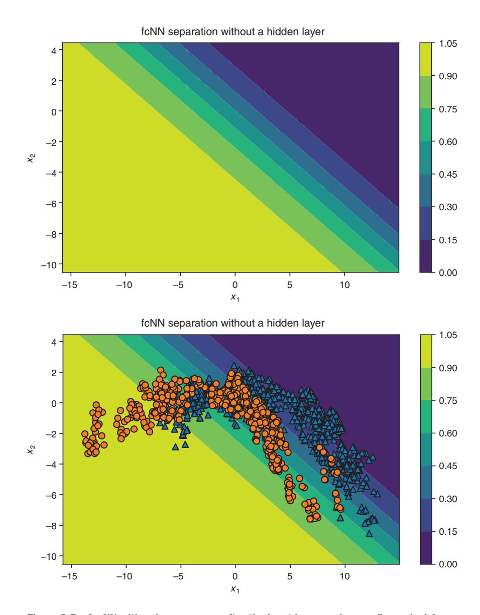
{alt=”Figure 2.7 An NN with only one neuron after the input layer produces a linear decision boundary. The shading of the background in the 2D feature space shows the probability for a fake banknote. The right side overlays the training data, showing that the linear decision curve doesn’t fit nicely in the boundary between the real and fake banknotes.”}

for the first class and the other neuron modeling the probability for the second class. This output layer design generalizes to classification tasks with more than two classes. In this case, the output layer has as many neurons as you have classes in the classification

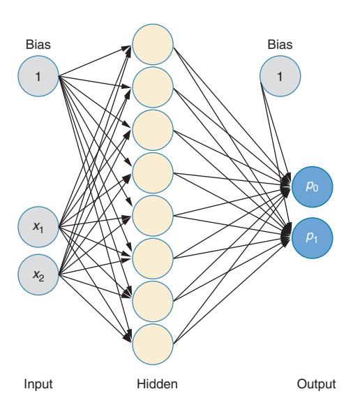
{alt=”Figure 2.8 An fcNN with one hidden layer consisting of eight nodes. The input layer has two nodes corresponding to two features in the banknote data set, and the output layer has two nodes corresponding to two classes (real and fake banknotes).”}

problem. Each neuron stands for a class, and you want to interpret the output of the neuron as the probability for the class. This can be done using the softmax function. The softmax function takes the weighted sum zi and transforms it into a probability pi by setting .

This ensures that the values are between 0 and 1 and, further, add up to 1. You can therefore interpret pi as the probability for the class i. The “soft” in softmax indicates that, rather than giving a hard call to one of the possible classes, the network can assign smaller probabilities to the other classes.

The y vector of the training data also has to be changed to be compatible with the two outputs. It was y = 1 if the example belonged to the class fake and y = 0 for the class real. Now you want the label to describe the two possible outputs. A real banknote should have the output values p0 = 1 and p1 = 0, and a fake banknote, the values p0 = 0 and p1 = 1. This can be achieved by a one-hot encoding of y. You start with a vector with as many zeros as you have classes (here two). Then you set one entry to 1. For y = 0, you set the 0th entry to 1 so that you have the vector (1, 0), and for y = 1, you have the vector (0, 1). For the architecture of the fcNN, see figure 2.8, and for the corresponding Keras code, see listing 2.2.

Listing 2.2 Definition of the network with one hidden layer

model = Sequential()
model.add(Dense(8, batch_input_shape=(None, 2),
    activation='sigmoid'))
model.add(Dense(2, activation='softmax'))
# compile model
model.compile(loss='categorical_crossentropy',
    optimizer=sgd)

Definition of the hidden layer with eight neurons.
The output layer with two output neurons.

As you can see in figure 2.9, the network now yields a curved decision surface, and it’s better able to separate the two classes in the training data.

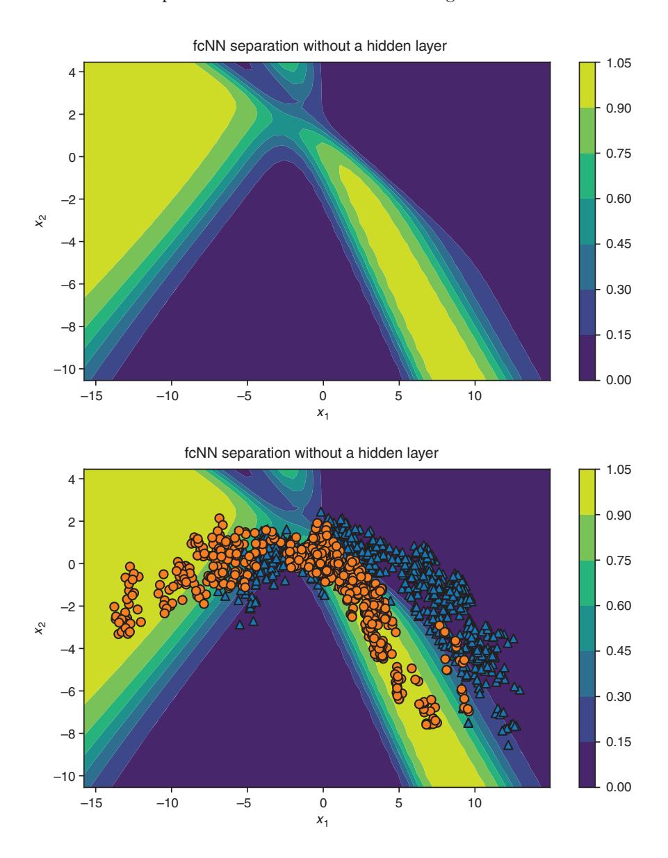
{alt=”Figure 2.9 An fcNN produces a curved decision boundary. The shading of the background in the 2D feature space shows the probability for a fake banknote predicted by an fcNN with one hidden layer that contains eight neurons and uses the features x1 and x2 as input. The right side overlays the training data, showing that the curved decision boundary better fits the boundary between the real and fake banknotes.”}

{alt=”Screenshot related to the hands-on time section for adding more hidden layers.”}

HANDS-ON TIME Become a member of the DL club by just adding more hidden layers in the banknote notebook (http://mng.bz/lGd6). It’s much easier than machine learning (see figure 2.10).

{alt=”Figure 2.10 A DL expert at work. Inspired by http://mng.bz/VgJP.”}

But what’s going on when adding an additional layer? In principle, the same thing as we discussed for the first hidden layer. You can see the neuron values in the added hidden layer as a new feature representation of the input. But there’s one difference: the features in deeper layers aren’t directly constructed from the input but from the previous layer. For example, in the second hidden layer, the features are constructed from the features in the first hidden layer (see figure 2.12). This hierarchical construction of the features is often efficient because it allows you to learn from the first layer basic features that can be used as components in several more complex features of the next layer.

The good news in DL is that you don’t need to predefine weights that determine how to construct the features in one layer from the features in the previous layer. The NN learns this during the training. You also don’t need to train each layer separately, but you usually train the NN as a whole, which is called end-to-end training. This has the
advantage that changes in one layer automatically trigger adaptations in all other layers. In chapter 3, you’ll learn how this training process works.

2.1.3 Using a fully connected NN (fcNN) to classify images

Let’s now use your new skills to build a larger network and see how it performs on the task of classifying handwritten digits. Different scientific disciplines have different model systems that benchmark their methods: molecular biologists use a worm called C. Elegance; people performing social network analysis use the Zachary Karate Club, and finally, people working with DL use the famous MNIST digit data set. This benchmark data set consists of 70,000 handwritten digits and is available from http://mng.bz/xW8W. The images all have 28 × 28 pixels and are grayscaled with values between 0 and 255. Figure 2.11 displays the first four images of the data set.

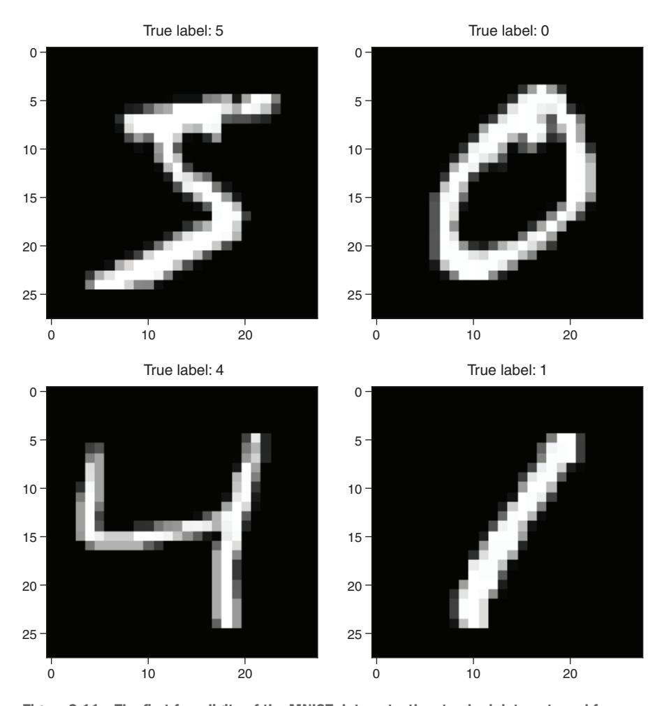
Figure 2.11 The first four digits of the MNIST data set—the standard data set used for benchmarking an NN for image classification.

This data set is well known in the machine learning community. If you develop a novel algorithm for image classification, you usually also report its performance on the MNIST data set. The MNIST images are grayscale images, and the gray value of each pixel is defined by an integer in the range from 0 to 255. For a fair comparison, there’s a standard split of the data: 60,000 of the images are used for training the network and 10,000 are used for testing. In Keras, you can download the whole data set with a single line (see listing 2.3). You can also download the companion MNIST notebook for this section (on which you can work later) at http://mng.bz/AAJz.

Simple neural networks can’t deal with 2D images but need a 1D input vector. Hence, instead of feeding the 28 × 28 images directly, you first flatten the image into a vector of size 28 · 28 = 784. The output should indicate whether the input image is one of the digits 0–9. More precisely, you want to model the probability that the network thinks that a given input image is a certain digit. For this, the output layer has ten neurons (one for each digit). You again use the activation function softmax to ensure that the computed outputs can be interpreted as probabilities (numbers between 0 and 1), adding up to 1. For this example, we also include hidden layers. Figure 2.12 shows a simplified version of the network and the definition of the corresponding model in Keras is shown in listing 2.4.

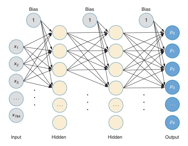
Figure 2.12 An fcNN with two hidden layers. In the MNIST example, the input layer has 784 values for the 28 × 28 pixels and the output layer has 10 nodes for the 10 classes.

Listing 2.3 Loading the MNIST data

from tensorflow.keras.datasets import mnist
(x_train, y_train), (x_test, y_test) = 
    mnist.load_data()
X_train = x_train[0:50000] / 255
Y_train = y_train[0:50000]
Y_train = to_categorical(Y_train, 10)
X_val = x_train[50000:60000] / 255

• mnist.load_data(): Loads the MNIST training (60,000 images) and test set.
• X_train = x_train[0:50000] / 255: Uses 50,000 images for training, dividing by 255 so that the pixel values are in the range 0 to 1.
• Y_train = to_categorical(Y_train, 10): Stores the labels given as integers from 0 to 9 as one-hot encoded vectors.
• X_val = x_train[50000:60000] / 255: We do the same with the validation set.

NOTE We don’t use the test set for this listing.

Also, where we store the labels for the $y_{train}$ for the network, we transform those to categorical data of length 10 to match the output. A 1 is translated as (0,1,0,0,0,0,0,0,0,0,0). This is called one-hot encoding. In the next listing, you can see a small fcNN using the one-hot encoded labels $y_{train}$.

Listing 2.4 Definition of an fcNN for the MNIST data

model = Sequential()
model.add(Dense(100, batch_input_shape=(None, 784),
                      activation='sigmoid'))
model.add(Dense(50, activation='sigmoid'))
model.add(Dense(10, activation='softmax'))
model.compile(loss='categorical_crossentropy',
              optimizer='adam',
              metrics=['accuracy'])
history = model.fit(X_train_flat, Y_train,
                    batch_size=128,
                    epochs=10,
                    validation_data=(X_val_flat, Y_val))

• model.add(Dense(100, ...)): The first hidden layer with 100 neurons, connected to the input size 28 x 28 pixels.
• model.add(Dense(50, ...)): A second dense layer with 50 neurons.
• model.add(Dense(10, ...)): The third layer connecting to the 10 output neurons.
• optimizer='adam': Uses a different optimizer than the SGD, which is faster (see chapter 3).
• history=model.fit(...): Tracks the accuracy (fraction of correctly classified training and validation examples) during the training.

HANDS-ON TIME Now open the MNIST notebook http://mng.bz/AAJz, run it, and try to understand the code.

When looking at the course of the loss curves over the number of iterations (figure 2.13), you can observe that the model fits the data. The performance of the trained fcNN on the validation set is around 97%, which isn’t bad, but the state of the art is about 99%.

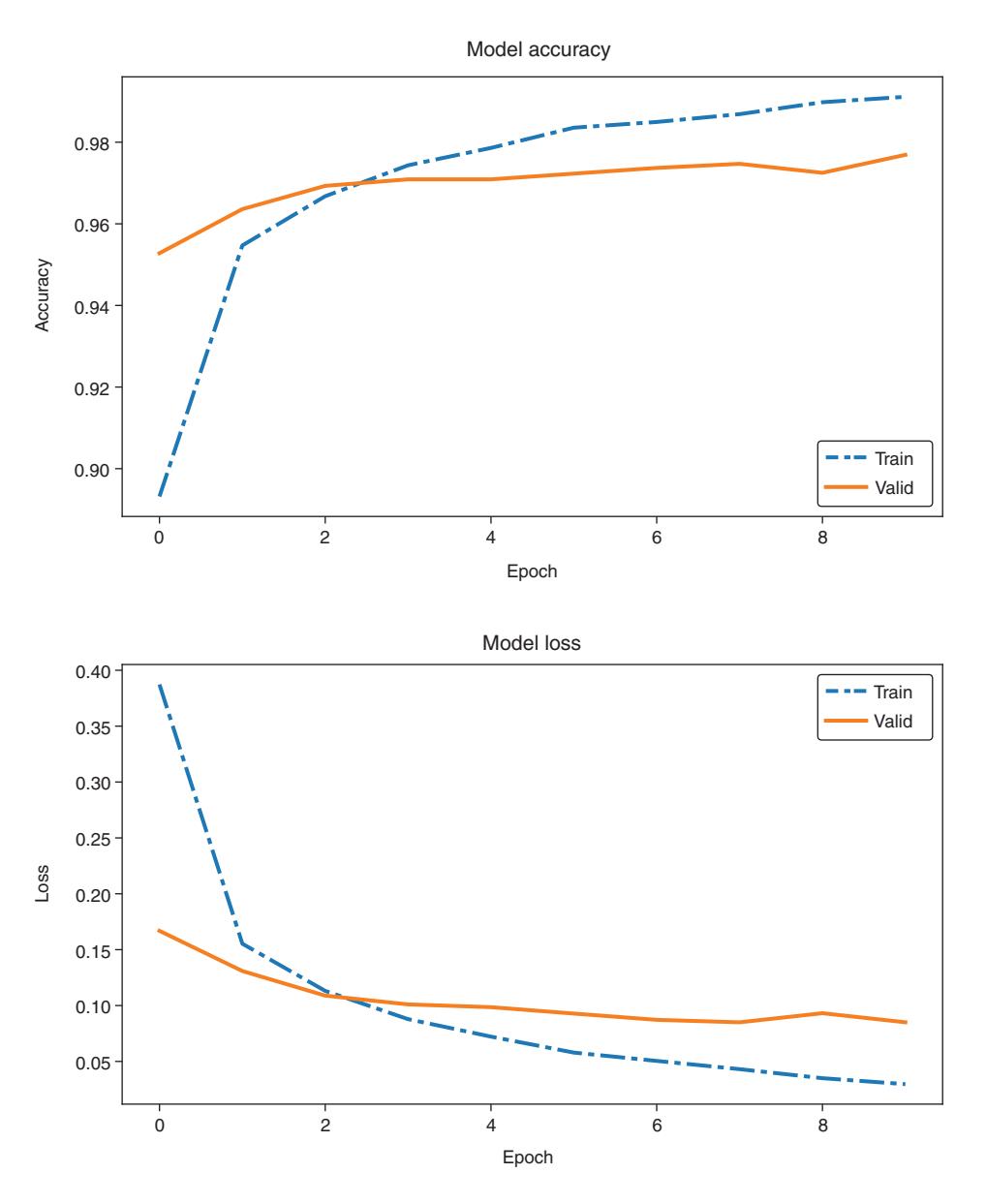
and loss decrease (bottom) during training”)

Figure 2.13 The increase of the accuracy training (top) and the decrease of the loss (bottom) during the different training steps

Play the DL game and stack more layers. Another trick that’s often used is to replace the sigmoid activation function in the hidden layers with something easier: ReLU. ReLU stands for Rectified Linear Unit and is quite a mouthful for what it really does. It simply clamps values smaller than zero to zero and leaves values larger than zero as they are (see figure 2.14). It is essential to use non-linear activation functions in

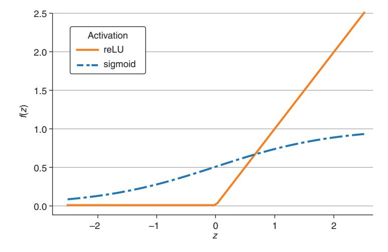
Figure 2.14 A comparison between the ReLU and the sigmoid activation functions

hidden layers, because when using a linear activation function, you can replace a stack of layers by only one layer. (This is because going through a linear layer corresponds to a matrix multiplication, and you can replace a series of matrix multiplications by one matrix multiplication.) To change the activation in Keras, simply exchange sigmoid with relu. If you like, you can change the activation function in the notebook http://mng.bz/AAJz.

Let’s do a small experiment and investigate what happens if you shuffle the pixel values before you feed those into the network. Figure 2.15 shows the same digits as in figure 2.11, but this time randomly shuffled.

For each image, the pixels have been shuffled the same way. You’d have a hard time telling the right digit even after seeing thousands of training examples. Can a network still learn to recognize the digits?

HANDS-ON TIME Try it out and play with the code in the MNIST notebook http://mng.bz/2XN0. What do you observe?

NOTE Only follow the notebook until you reach the section “CNN as a classification model for MNIST data.” We’ll look at CNNs later and then revisit the notebook.

You’ll probably reach the same accuracy (within statistical fluctuations) as with the original images. This might come as a surprise at first. But looking at the network architecture of an fcNN, the order of the input doesn’t matter whatsoever. Because the network has no concept of nearby pixels, there’s nothing like a neighborhood. People, therefore, also call fcNN permutation invariant NN because its performance

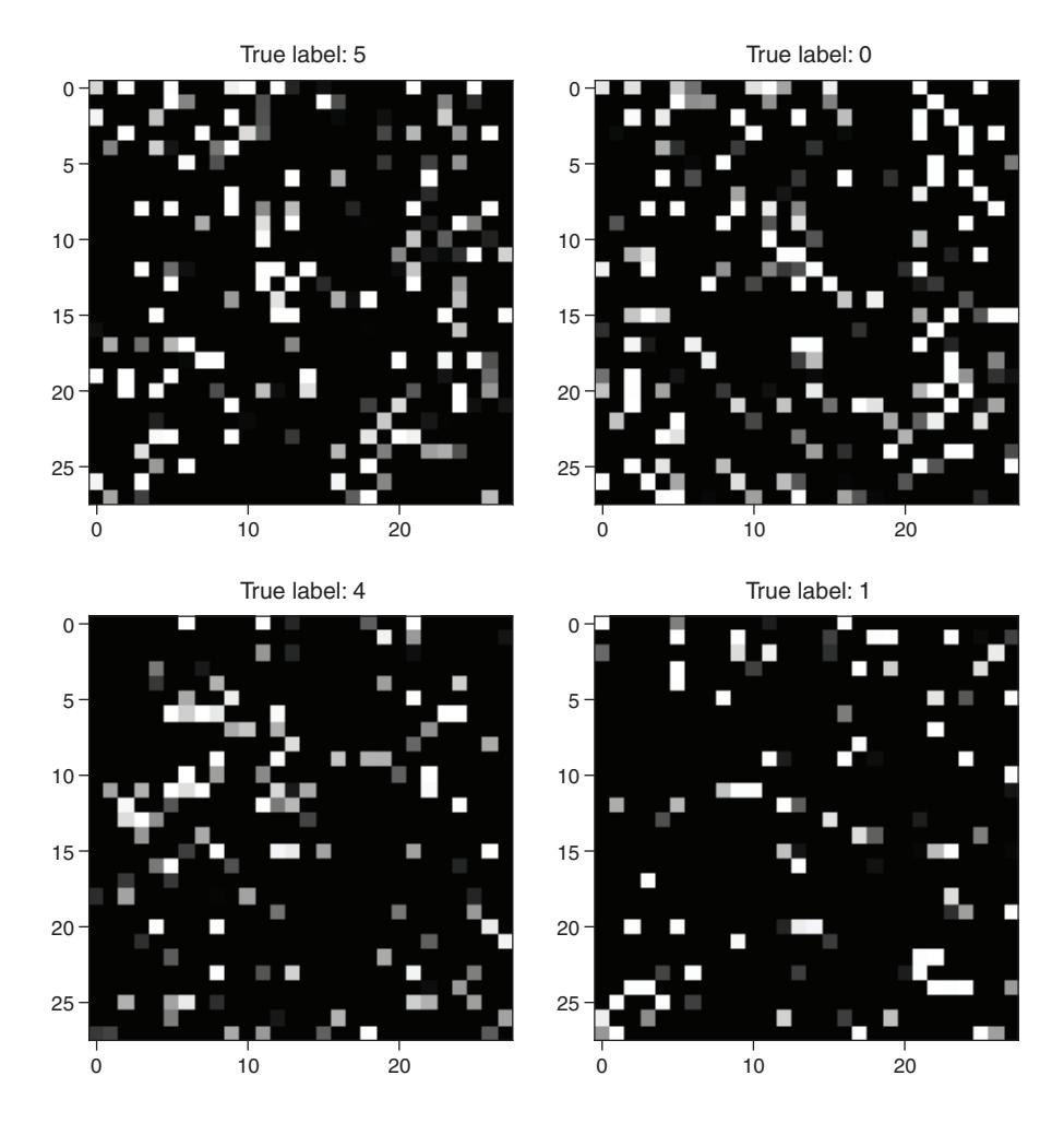
with pixels randomly shuffled”)

Figure 2.15 The same digits (5, 0, 4, 1) as in figure 2.11 after shuffling the pixels

doesn’t depend on whether the data is permuted (shuffled). However, real image data isn’t permutation invariant, and nearby pixels tend to have similar values. If you shuffle images, people will have a problem recognizing those. Moreover, two images showing the same digit don’t need to show the same pixel values. You can move (translate) the image a bit, and it still shows the same object.

The fact that humans are great in visual tasks but have problems with shuffled images indicates that the evolution has found ways to take advantage of the special properties of image data. While fcNNs are good for spreadsheet-like data where the order of the columns doesn’t matter, there are better architectures when the order or the spatial alignment does matter, like convolutional NNs. In principle, fcNN can be used for images, but you need many layers and huge training data sets that allow the

network to learn that nearby pixels tend to have the same values and that images are translation invariant.

2.2 Convolutional NNs for image-like data

Fully connected NNs with even a single hidden layer can represent any function, but quickly get too big and contain so many parameters that you usually don’t have enough data to fit them. Much of the progress in DL has been around creating different architectures that more efficiently exploit the structure of the data. For image data, one such architecture is convolutional NNs.

For the example of an fcNN with only one hidden layer (see figure 2.8), we discussed that you can view the number of neurons in the hidden layer as the number of new features that are constructed from the input. This implies that you need a large number of neurons in the hidden layer if you want to tackle a complex problem. But the more neurons you have in the hidden layer, the more parameters you need to learn, and the more training data you need. Stacking layers lets the model learn taskspecific features in a hierarchical manner. This approach needs fewer parameters than an fcNN to construct complex features and, therefore, is less data hungry.

You learned in the last section that you get more out of an fcNN if you add more hidden layers. Going deep is a great trick to enhance the performance of NNs, giving DL its name. You also learned that an fcNN ignores the neighboring structure of pixels in an image. This suggests that there might be a better NN architecture to analyze image data. And indeed, the success of DL in the field of computer vision was not possible without some additional architectural tricks that exploit the knowledge about the local structure of image data.

The most important ingredient to tailor an NN for locally correlated data such as image data is the so-called convolutional layers. In this section, we explain how a convolutional layer works. NNs that consist mainly of convolutional layers are called convolutional neural networks (CNNs) and have an extremely broad range of applications including:

• Image classification, such as discriminating a truck from a road sign
• Video data prediction, such as generating future radar images for weather forecasting
• Quality control in production lines based on image or video data
• Classification and detection of different tumors in histopathological slices
• Segmentation of different objects in an image

2.2.1 Main ideas in a CNN architecture

Let’s focus on image data and discuss a specialized NN architecture that takes into account the highly local structure within an image (see figure 2.16). In 2012, Alex Krizhevsky used this architecture in the internationally renowned ImageNet competition, which brought with it a breakthrough for DL into the field of computer vision.

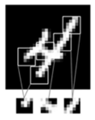
Figure 2.16 An image can be broken into local patterns such as edges, textures, and so on.

We’ll now dive into the architecture of CNNs and discuss how they got their name. Let’s look at the main idea of a CNN: instead of connecting all neurons between two successive layers, only a small patch of neighboring pixels connects to a neuron in the next layer (see figure 2.17). With this simple trick, the network architecture has the local structure of images built in. This trick also reduces the number of weights in the NN. If you only consider small patches of, for example, 3 × 3 pixels as a local pattern (see figure 2.18) that’s connected to a neuron in the next layer, then you have only weights to learn for the weighted sum , which is the input to the next neuron.

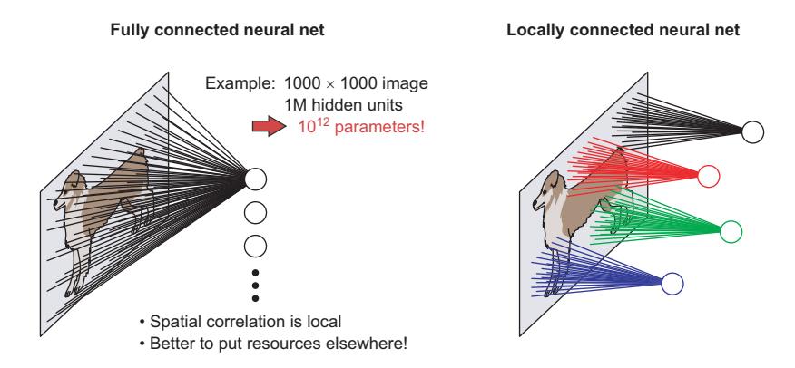
Figure 2.17 Connectivity between the input image and a neuron in the first hidden layer for an fcNN (on the left) or for a CNN (on the right). This representation ignores the bias term.

If you have experience with classical image analysis, then you know that this idea isn’t new at all. What you’re doing here is called convolution.

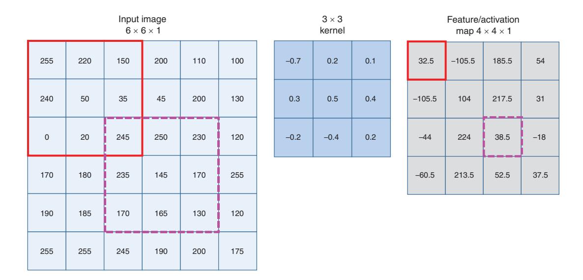
Figure 2.18 Convolution of a $6 times 6$ grayscale image with a $3 times 3$ kernel and a stride of 1 without padding yields as output a $4 times 4$ feature map. The kernel is applied at all 16 possible positions to determine the 16 values of the activation map. Two possible kernel positions are marked in the input with thick solid and dashed borders. The respective positions of the resulting pixels in the activation map are also marked with thick solid and dashed borders. The CNN computes the resulting values by multiplying the pixel values with the overlaid kernel values and adding all terms (bias is assumed to be 0).

Have a look at figure 2.18, where you see a small image with $6 times 6$ pixels and a $3 times 3$ kernel[^1] with predefined weights. You can slide the kernel over the image by taking steps of 1 pixel (called stride=1). At each position, you compute the element-wise multiplication of the image pixel and the overlaid kernel weights. You then add these values to get the weighted sum $z = x_1 cdot w_1 + x_2 cdot w_2 + ldots + x_k cdot w_k + b$, where k is the number of pixels connected to each neuron and b is a bias term. The computed value z is a single element of the output matrix. After shifting the kernel to the next position over the image, you can compute the next output value z and so on. We call the resulting output an activation map or feature map.

In the example in figure 2.18, we start with a $6 times 6$ image, convolve it with a $3 times 3$ kernel, and receive a $4 times 4$ activation map. Sliding a kernel over an image and requiring that the whole kernel is at each position completely within the image yields an activation map with reduced dimensions. For example, if you have a $3 times 3$ kernel on all sides, one pixel is knocked off in the resulting activation map; in case of a $5 times 5$ kernel, 2 pixels would be knocked off. If you want to have the same dimension after applying the convolution, you can use a zero padding of the input image (called padding=’same’, the argument of the convolution layer in listing 2.5; if you don’t want zero padding, the argument would be padding=’valid’).

[^1]: People in the field of DL and computer vision use the word kernel, but sometimes you also see the term filter, which can be used as a synonym.

In CNNs, the kernel weights are learned (see chapter 3). Because you use the same kernel at each position, you have shared weights, and in our example, you only need to learn weights to compute a whole activation map. Usually a bias term is also included in case there are 10 weights to learn. To interactively apply different kernels to a real image, see http://setosa.io/ev/image-kernels/.

What can the values in an activation map tell you? If you apply a kernel to all possible positions within the image, you get only a high signal where the underlying image shows the pattern of the kernel. Assembling the outputs to an image yields a map that shows at which positions in the image the kernel pattern appears. This is the reason why the resulting image is often called a feature map or an activation map.

Each neuron in the same activation map has the same number of input connections, and the connecting weights are also the same. (You’ll soon see that real applications use more than one kernel.) Each neuron is connected to a different patch of the input (previous layer), meaning that each neuron within the same feature map looks for the same pattern but at different positions of the input. Figure 2.19 demonstrates this concept for an abstract image that consists of rectangular areas where a kernel with a vertical edge pattern is applied. We use this technique in image manipulation, for example, to enhance the edges of an image or to blur it. Visit http://setosa.io/ev/image-kernels/ to get a feel for the effect of different kernels on more complex images.

In figure 2.19, you see the vertical-edge kernel (going from bright to dark) in three positions of the image. At an image position with a vertical edge that goes from bright to dark, you get a high value (shown as dark gray pixels in the activation map). At an image position with a vertical edge that goes from dark to bright, you get a low value (shown as light gray pixels in the activation map). At positions where there’s no vertical edge in the image, the resulting values are neither high nor low (shown as midgray pixels in the activation map). In case of the displayed filter where the weights add up to one, the values in the activation maps are zero if the input is an image patch with a constant gray value.

2.2.2 A minimal CNN for edge lovers

Let’s imagine an art lover who gets excited if an image contains vertical edges. Your task is to predict for a set of striped images if the art lover will like those. Some of the images in the set have horizontal edges and some vertical edges. To identify the images with vertical stripes, a vertical-edge detection model would be great. For this purpose, you might want to do something similar to that depicted in figure 2.19 and perform a convolution of a predefined vertical-edge filter, using the maximal value in the resulting feature map as a score that indicates if the art lover will like the image.

Using a predefined kernel for convolution is often done in traditional image analysis when the feature of interest is known and can be described as a local pattern. In

Image Feature/activation map

Kernel
0.16	-0.08	-0.08
0.16	-0.08	-0.08
0.16	-0.08	-0.08

6.00	6.00	6.00	6.00	6.00	6.00	16.00	16.00	16.00	16.00	16.00	16.00	16.00	16.00	16.00	16.00
6.00	6.00	6.00	6.00	6.00	6.00	16.00	16.00	16.00	16.00	16.00	16.00	16.00	16.00	16.00	16.00
6.00	6.00	6.00	6.00	6.00	6.00	16.00	16.00	16.00	16.00	16.00	16.00	16.00	16.00	16.00	16.00
6.00	6.00	6.00	6.00	6.00	6.00	16.00	16.00	16.00	16.00	16.00	16.00	16.00	16.00	16.00	16.00
22.00	22.00	22.00	22.00	22.00	22.00	16.00	16.00	16.00	16.00	16.00	16.00	16.00	16.00	16.00	16.00
22.00	22.00	22.00	22.00	22.00	22.00	16.00	16.00	16.00	16.00	16.00	16.00	16.00	16.00	16.00	16.00
22.00	22.00	22.00	22.00	22.00	22.00	16.00	16.00	16.00	16.00	16.00	16.00	16.00	16.00	16.00	16.00
22.00	22.00	22.00	22.00	22.00	22.00	16.00	16.00	16.00	16.00	16.00	16.00	16.00	16.00	16.00	16.00
22.00	22.00	22.00	22.00	22.00	22.00	16.00	16.00	16.00	16.00	16.00	16.00	16.00	16.00	16.00	16.00
22.00	22.00	22.00	22.00	22.00	22.00	3.00	3.00	3.00	3.00	3.00	3.00	3.00	3.00	3.00	3.00
22.00	22.00	22.00	22.00	22.00	22.00	3.00	3.00	3.00	3.00	3.00	3.00	3.00	3.00	3.00	3.00
22.00	22.00	22.00	22.00	22.00	22.00	3.00	3.00	3.00	3.00	3.00	3.00	3.00	3.00	3.00	3.00
22.00	22.00	22.00	22.00	22.00	22.00	3.00	3.00	3.00	3.00	3.00	3.00	3.00	3.00	3.00	3.00
22.00	22.00	22.00	22.00	22.00	22.00	3.00	3.00	3.00	3.00	3.00	3.00	3.00	3.00	3.00	3.00
22.00	22.00	22.00	22.00	22.00	22.00	3.00	3.00	3.00	3.00	3.00	3.00	3.00	3.00	3.00	3.00
22.00	22.00	22.00	22.00	22.00	22.00	3.00	3.00	3.00	3.00	3.00	3.00	3.00	3.00	3.00	3.00

Figure 2.19 Convolution of a 3 × 3 kernel with a weight pattern that resembles a vertical edge (upper left panel) with an image consisting of squared areas (lower left and right panel) results in a feature map that highlights the positions of vertical edges in the input image (upper right panel). In the left panel, the numbers indicate the weighted values for the kernel (upper left) and the pixel values for the image (lower left).

such a situation, it’d be rather silly not to use this traditional image analysis approach. But let’s pretend you don’t know that the art lover likes vertical edges, and you only have a list of images that they like and dislike. You want to learn the values for the weights within the kernel that you can use for convolution. Figure 2.20 shows the corresponding network architecture, where the size of the kernel is 5 × 5. The resulting hidden layer is a feature map.

To check if this feature map indicates that the image contains the kernel pattern, you take the maximum value of the feature map. From this value, you want to predict

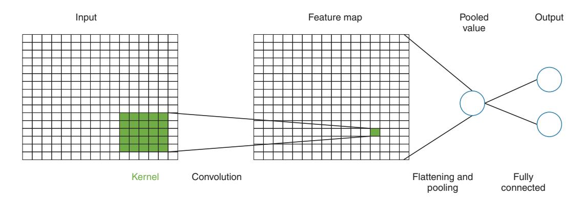
Figure 2.20 A CNN with only one hidden layer consisting of one feature map. As a pooled value, you take a maximum of all values within the feature map. You add a dense layer to determine the probability for two possible class labels in the output.

the probability that the art lover likes the image. You already saw how to do that: you add a single, fully connected layer with two output nodes and use softmax activation to ensure that the two output values can be taken as probabilities for the two classes (art lover likes the image; art lover doesn’t like the image). This adds up to 1. This small CNN network (the feature map in the first hidden layer) results from the convolution of the image with a kernel. The classification is done in the fully connected part shown on the right side in figure 2.20. This architecture is probably one of the smallest possible CNNs one can think of. To model image data with TensorFlow and Keras, you need to create 4D tensors with the form:

(batch, height, width, channels)

The batch dimension corresponds to the number of images in one batch. The next two elements define the height and width of the image in units of pixels. The last dimension defines the number of channels. (A typical RGB color image has 3 channels. This means that a batch of 128 color images, each having 256 rows and columns, could be stored in a tensor of shape (128, 256, 256, 3.)

You can set up, train, and evaluate the CNN model with a few lines of Keras code (see listing 2.5). The only thing you need is a data set of images with horizontal or vertical stripes and a corresponding class label. This can be easily simulated.

{alt=”Figure 2.20: A simple CNN architecture, illustrating convolutional layers generating feature maps and fully connected layers for classification.”}

HANDS-ON TIME Open the edge lovers’ notebook at http://mng.bz/1zEj and follow the instructions there to simulate the image data and fit the model. Check out which kernel weights are learned and if these form a vertical edge. If you can’t reproduce the result, don’t worry; just do the training again until you get the result. Investigate the impact of the activation function and the pooling method.

Listing 2.5 Edge lovers’ CNN

model = Sequential()
model.add(Convolution2D(1,(5,5),padding='same',input_shape=(pixel,pixel,1)))
model.add(Activation('linear'))
# take the max over all values in the activation map
model.add(MaxPooling2D(pool_size=(pixel,pixel)))
model.add(Flatten())
model.add(Dense(2))
model.add(Activation('softmax'))
# compile model and initialize weights
model.compile(loss='categorical_crossentropy',
                optimizer='adam',
                metrics=['accuracy'])
# train the model
history=model.fit(X_train, Y_train,
                    validation_data=(X_val, Y_val),
                   batch_size=64,
                   epochs=15,
                    shuffle=True)

• The Convolution2D layer uses one kernel of size 5x5 with ‘same’ padding.
• A linear activation function is added, passing all values through.
• The MaxPooling2D layer extracts the maximal value of the feature map.
• The Flatten layer converts the output of the previous layer into a vector.
• A Dense layer with two neurons predicts the probabilities of two labels.
• A softmax activation function is used to compute probabilities for the two classes.

NOTE In the listing, using a convolutional layer with padding=’same’ means that the output feature map has the same size as the input image.

In your experiments with the edge lovers’ notebook at http://mng.bz/1zEj, you’ve probably seen that a vertical edge kernel isn’t always learned; sometimes a horizontal edge kernel is learned instead. This is perfectly fine because the data set consists of images with either horizontal or vertical edges, and the task is only to discriminate between horizontal and vertical edges. Finding no horizontal edges indicates that the image contains only vertical edges.

In this edge lovers’ example, it probably makes no difference if you use a predefined kernel or learn the weights of the kernel. But in a more realistic application, the best discriminating pattern is sometimes hard to predefine, and learning the optimal kernel weights is a great advantage of CNNs. In chapter 3, you’ll learn how the weights of a model are trained.

2.2.3 Biological inspiration for a CNN architecture

The edge lovers’ example was only a toy, and you might think that there’s certainly no edge-loving neuron in a real brain. The opposite is true! The so-called visual cortex in the brains of humans and animals, indeed, have such edge-loving neurons. Two biologists, Hubel and Wiesel, received the Nobel prize in Physiology or Medicine for discovering this in 1981. The way they found this is quite interesting. And, as is often in research, there is a great deal of luck involved.

In the late 1950s, Hubel and Wiesel wanted to investigate the correlation of the neuronal activity due to stimuli in the visual cortex of a cat. For this purpose, they anesthetized a cat and projected some images on a screen in front of it. They picked a single neuron to measure the electrical signal (see figure 2.21). The experiment, however, seemed not to work because they couldn’t observe the neuron firing while presenting different images to the cat. They changed the slides in the projector to those of an increasingly higher frequency. Finally, they shook the projector because a slide got stuck and then the neuron started to fire. In this manner, they discovered that neurons in different positions in the visual cortex are activated if edges with different orientations slide over the retina of the cat’s eye.

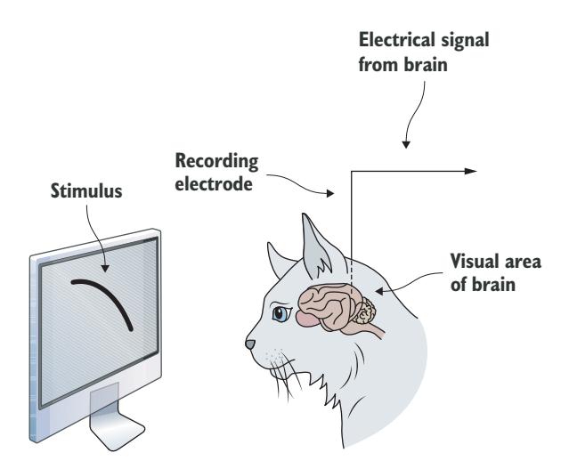
{alt=”Figure 2.21 Setup of the experiment of Hubel and Wiesel in which they discovered neurons in the visual cortex that responded when they showed moving edges to a cat.”}

Figure 2.21 Setup of the experiment of Hubel and Wiesel in which they discovered neurons in the visual cortex that responded when they showed moving edges to a cat.

Brain research continued to develop, and now it’s widely known that in the area of the brain where Hubel and Wiesel did their experiments (called the V1 region), all neurons respond to rather simple forms of stimuli on different areas of the retina. This isn’t only true for cats but also for other animals and humans. It’s also known that neurons in other regions of the brain (called V2, V4, and IT) respond to increasingly complex visual stimuli like, for example, a whole face (see figure 2.22). Research shows that a neuron’s signal is transmitted from region to region. Also, only parts of the neurons in one region of the brain connect to the neurons in the next region. Via the connections of the neurons, the activation of different neurons is combined in a hierarchical way that allows the neurons to respond on increasingly larger regions in the retina and to more and more complex visual stimuli.

NOTE You’ll see soon that the architecture of deeper CNNs are loosely inspired by this hierarchical detection of complex structures from simple

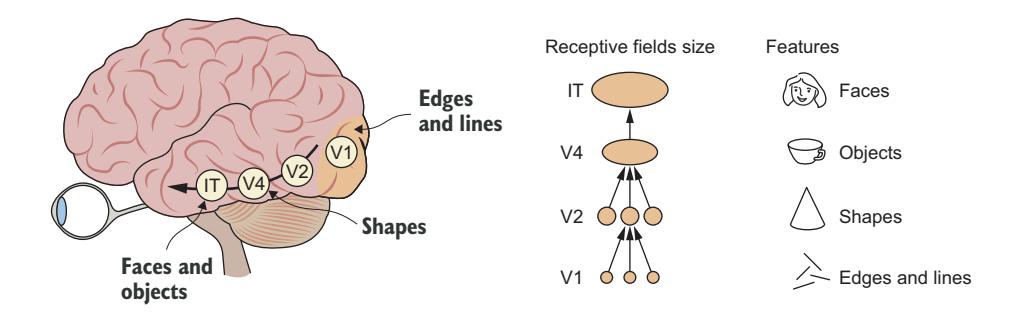
{alt=”Figure 2.22 Organization of the visual cortex in a brain. Neurons in different regions respond to an increasingly larger receptive field and more and more complex stimuli.”}

Figure 2.22 Organization of the visual cortex in a brain. Neurons in different regions respond to an increasingly larger receptive field and more and more complex stimuli.

structures. However, the analogy shouldn’t be overstressed; the brain isn’t wired up to form a CNN.

2.2.4 Building and understanding a CNN

More realistic image classification tasks can’t be tackled by such a simple CNN architecture such as that depicted in figure 2.20, which only learns to detect one local image pattern like an edge. Even simple image classification tasks like discriminating between the 10 digits in the MNIST data set require learning lots of more complex image features. You can probably already guess how to do that: going deep is the main secret. But before going deep, you need to go broad and add more kernels to the first layer.

Each kernel can learn another set of weights, and so for each kernel, you get another activation map in the hidden layer (see figure 2.23). If the input has not only 1 but d channels, then the kernel also needs to have d channels to compute an activation map. For color images, d = 3 for (red, green, blue), and a valid kernel can be one that is active for a vertical edge in the green channel and for horizontal edges in the blue and red channels. The kernel matrix again defines the weights for the weighted sum, which determines the input to the neuron in the respective position of the activation map.

Now let’s talk about analogies between fcNNs and CNNs. An fcNN learns a new set of weights for each neuron (the learning process is discussed in chapter 3) that combines the input of the former layer to a new value that can be seen as a feature of the image (see, for example, figure 2.8). In an fcNN, you can go deep by adding layers where all neurons of one layer are connected to all neurons in the next layer. In this sense, the number of kernel sets or activation maps in a CNN correspond to the number of neurons in one layer of an fcNN. If you want to go deep in a CNN, you need to add more convolutional layers. This means that you learn kernels that are again applied to the stack of activation maps of the previous layers.

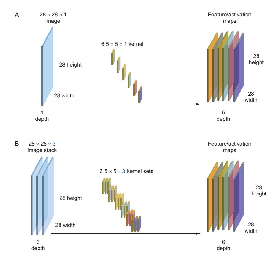
{alt=”Figure 2.23 Convolution of the input image with six different kernels results in six activation maps. If the input image has only one channel (a), then each kernel has also only one channel. If the input image has three channels (b), then each filter has also three channels.”}

Figure 2.23 Convolution of the input image with six different kernels results in six activation maps. If the input image has only one channel (a), then each kernel has also only one channel. If the input image has three channels (b), then each filter has also three channels.

Figure 2.25 illustrates this principle. In that figure, you see a CNN with 3 convolutional layers. The convolution over a stack of activation maps isn’t different than the convolution with an input of several channels. In figure 2.23, only 6 activation maps are generated from a 3-channel input image. However, learning only 6 kernels isn’t common. A typical number to learn is 32 kernels in the first layer or even more kernels. (Often the number of kernels doubles when moving from layer to layer.) To reduce the number of weights in a CNN, it’s also common to downsample the activation maps before doing the next round of convolution. This is often done by replacing a $2 times 2$ patch of neurons in an activation map with the maximal activation. We call this step max pooling.

When adding more layers to a CNN, the area that a neuron sees in the original image gets larger. We call this a receptive field, and it’s composed of all the pixels in the original image to which the neuron is connected, through all intermediate layers.

Depending on the image size and the kernel size (often after around four to ten layers), all neurons connect to the whole input image. Still, the complexity of image patterns that activate the neurons in different layers of the CNN gets higher with each layer.

When checking which images or image parts can activate a neuron in the different layers of a CNN, layers close to the input respond to simple image patterns (like edges) and layers close to the output combine these simple patterns into more complex patterns (see figure 2.24).

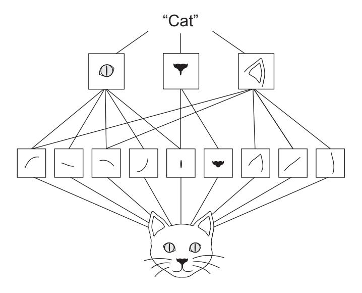
The number of convolutional layers and the numbers of kernels within each layer are tuning parameters in a CNN. When the complexity of the problem increases, you usually need more convolutional layers and more kernels per layer. In the last convolutional layer of the CNN, we have a new representation of the input. Flattening all neurons of this layer into a vector results in a new feature representation of the image with as many features as there were neurons in the last convolutional layer (see figure 2.25). We end up with the same situation as before: the input is described by a vector of image features. But this time, the features are results from trained kernels. Now you can add a couple of densely connected layers to construct the prediction.

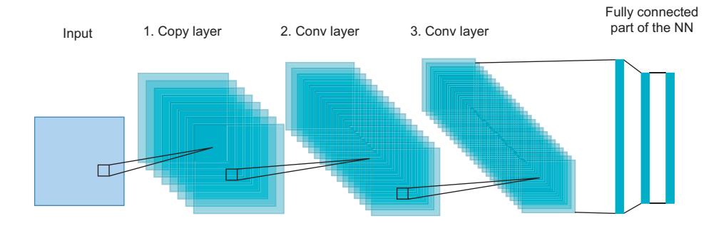
Figure 2.25 A CNN with three convolutional layers followed by three fully connected layers. The number of feature maps in each convolutional layer indicate the number of kernel sets learned. The number of elements in each layer of the fully connected part indicate the number of weighted sets learned.

Let’s try a CNN on the MNIST data. In listing 2.6, you see the definition of a CNN with convolutional layers followed by fully connected layers.

HANDS-ON TIME Open the MNIST notebook again http://mng.bz/AAJz and fit a CNN with two convolutional layers to the MNIST data (see the second part of the notebook). Then compare the performance to what you achieved with an fcNN. Play with the code and perform a permutation experiment to check that the order of the pixels within the images matter for the performance of the CNN.

Listing 2.6 A CNN for MNIST classification

# define CNN with 2 convolution blocks and 2 fully connected layers
model = Sequential()
model.add(Convolution2D(8, kernel_size,
                        padding='same', input_shape=input_shape))
# Uses a convolutional layer with eight kernels of the size 3 times 3
model.add(Activation('relu'))
# Applies the relu activation function to the feature maps
model.add(Convolution2D(8, kernel_size, padding='same'))
model.add(Activation('relu'))
model.add(MaxPooling2D(pool_size=pool_size))
# This max pooling layer has a pooling size of 2 times 2 and a stride of 2.
model.add(Convolution2D(16, kernel_size, padding='same'))
# Uses a convolutional layer with 16 kernels of the size 3 times 3
model.add(Activation('relu'))
model.add(Convolution2D(16, kernel_size, padding='same'))
model.add(Activation('relu'))
model.add(MaxPooling2D(pool_size=pool_size))
# This max pooling layer transforms the 14 times 14 times 16 input tensor
# into a 7 times 7 times 16 output tensor.
model.add(Flatten())
# Flattens the output of the previous layer resulting in a
# vector of length 784 (7 times 7 times 16)
model.add(Dense(40))
model.add(Activation('relu'))
model.add(Dense(nb_classes))
# Outputs nb_classes (here 10)
model.add(Activation('softmax'))
# Uses softmax to transform the 10 outputs to 10 prediction probabilities

# compile model and initialize weights
model.compile(loss='categorical_crossentropy',
              optimizer='adam',
              metrics=['accuracy'])
# train the model
history = model.fit(X_train, Y_train,
                    batch_size=128,
                    epochs=10,
                    verbose=2,
                    validation_data=(X_val, Y_val)
                    )

The first convolutional layer with eight kernels with the same padding results in an output feature map that has the same size as the input image. In the MNIST case, the input image has a size 28 × 28 × 1 pixels. The resulting eight feature maps each have a size of 28 × 28. After the first pooling, the input has a shape of 28 × 28 × 8, and the output has a shape of 14 × 14 × 8.

From your experiments with the MNIST notebook at http://mng.bz/AAJz, you’ve learned that with this image classification task, it’s easy to achieve a higher performance with a CNN (around 99%) than with an fcNN (around 96%). The permutation experiment shows that the arrangement of the pixels within the image does matter: the CNN performs much better when trained on the original image data (99%) than when trained on a shuffled version of the image data (95%). This supports the idea that the secret of the high performance of a CNN in image-related tasks lies in the architecture that takes the local order of an image into account. Before moving on, let us look back and emphasize some advantages of CNNs when working with image data:

• Local connectivity makes use of the local information of image data.
• You need less weight parameters in a CNN than in an fcNN.
• A CNN is to a large extent invariant to translations within the images.
• The convolutional part of a CNN allows the network to learn hierarchically task-specific abstract image features.

The next special case of data that’s successfully analyzed with DL is data that shows an ordering. Let’s look at that next.

2.3 One-dimensional CNNs for ordered data

Ordered data can be text (understood as sequences of words or characters), time series (like the daily maximum temperature in Zürich), sound, or any other data that’s ordered. Applications of these algorithms include the following:

• Document and time series classification, such as identifying the topic of an article or the author of a book
• Sequence comparisons, such as estimating how closely related two documents or two stock tickers are
• Sequence-to-sequence learning, such as decoding an English sentence into French
• Sentiment analysis, such as classifying the sentiment of tweets or movie reviews as positive or negative
• Time series forecasting, such as predicting the future weather at a certain location given recent weather data

2.3.1 Format of time-ordered data

To model sequential data with TensorFlow and Keras, you need to provide that data as 3D tensors:

(batch, timestep, input_feature)

The batch dimension specifies the number of sequences that are processed in one batch. Using many sequences in a batch is only for performance reasons. The sequences in a batch are processed independently. This is the same situation as with the previous CNNs, where the images in a batch are also processed independently. When calculating the loss function, the results of those different sequences in a batch are averaged.

Let’s look at an example. You want to predict the daily maximum temperature for tomorrow. You have 12 years of historical data, and you want to take the last 10 days into account to predict tomorrow’s temperature. You choose a batch size of 128. In that case, the input tensor has the following shape: (128, 10, 1). Let’s refine the model. Maybe there’s information in the daily maximum temperature of five nearby cities that can help with your prediction. You also take those temperatures into account, which results in an input tensor of shape (128, 10, 6).

Another application area of ordered data is text analysis. Let’s say you want to analyze text with characters as input. The timestep dimension specifies the position of a character within a sequence. The input_feature dimension holds for each sequence and timestep the actual values.

Let’s take another example. Suppose you want to analyze text data in lowercase at the character level. The third sequence in the batch starts with “hello.” You could encode “hello” by using the position of the letters in the alphabet as (8, 5, 11, 11, 14). Coding characters like this implies an ordering that’s artificial. Therefore, in DL, categorical data is treated using one-hot encoding. See http://mng.bz/7Xrv for a more detailed description of one-hot encoding. The first two elements of this sequence in the 3D input tensor would then be:

input [2,0,:] = (0,0,0,0,0,0,0,1,0,0,0,0,0,0,0,0,0,0,0,0,0,0,0,0,0,0)
# a,b,c,d,e,f,g,h,i,j,k,l,m,n,o,p,q,r,s,t,u,v,w,z,x,z
#the 1 at position 8 indicates the 8th character in the alphabet, which is h
input [2,1,:] = (0,0,0,0,1,0,0,0,0,0,0,0,0,0,0,0,0,0,0,0,0,0,0,0,0,0)
# a,b,c,d,e,f,g,h,i,j,k,l,m,n,o,p,q,r,s,t,u,v,w,z,x,z
#the 1 at position 5 indicates the 5th character in the alphabet, which is e

One-hot encoding is useful if you need to model text at the character level when you have a limited number of characters. If you model text at the word level and do one-hot encoding, you need vectors with as many dimensions as you have words. These vectors would get quite large and sparse, and hence, it’s better to find a denser representation. This is a step we call embedding, which yields a new representation of the word as a vector of numbers. In chapter 6 of Chollet’s book at http://mng.bz/qMGr, you can find more details of transforming text to vectors and some demo code for Keras.

2.3.2 What’s special about ordered data?

For text and other ordered data, the sequences often have some particular properties. The first property is that there is often no notion of a natural starting point in time. Becoming a bit philosophical, if you forget about the Big Bang for now and consider normal time spans, there’s no marked starting point. This has as a consequence that all physical laws must be invariant in time. If you play table tennis, the trajectory of the ball is the same as in the 15th century. The second particularity is that time-ordered data often includes long-range dependencies. Consider the following string (taken from Wikipedia’s article on Kant, https://en.wikipedia.org/wiki/Immanuel_Kant):

Kant was born on April 22, 1724 into a Prussian German family of Lutheran Protestant faith in Königsberg, East Prussia. . . . [thousands of words left out]. A common myth is that Kant never traveled more than 16 kilometers (9.9 mi) from Königsberg his whole life. . . . [thousands of words left out]. Kant’s health, long poor, worsened and he died at ___.

What’s the probability of the next word being one of these: a) lightsaber, b) London, or c) Königsberg? This shows that there are quite long-range dependencies in sequential data. Also, lengthy range dependencies can be found in other ordered data. For example, if you consider the daily maximum temperature at an arbitrary place on earth, it’s quite likely that 365 data points later, a similar temperature occurs (at least more likely than 182 days later). The last special property of ordered data occurs especially in time series, where there’s a notion of past, present, and future. In this case, the future doesn’t have an impact on the past. This feature is true for a time series like the temperatures in a weather forecast but not for tasks in sentiment analysis.

An optimal network should incorporate these hard facts in its design so that it doesn’t need to learn them. In the case of causal networks, the architecture ensures that only information from the past has an influence on the present. Similarly, in the case of CNN for images, the architecture with shared weights ensures that the model is invariant to small spatial shifts.

2.3.3 Architectures for time-ordered data

We often analyze time-ordered data using so-called recurrent neural networks (RNNs) like long short-term memory networks (LSTMs). These networks are conceptually a bit more complicated than CNNs. Furthermore, RNNs are a bit harder to train. In many applications, RNNs can be replaced by CNNs, or as the finding of a recent research paper states it (Bai et al., https://arxiv.org/abs/1803.01271):

We conclude that the common association between sequence modeling and recurrent networks should be reconsidered, and convolutional networks should be regarded as a natural starting point for sequence modeling tasks.

Because you don’t need RNNs for the rest of the book, refer to chapter 6 of Chollet’s book at http://mng.bz/mBea, and proceed with CNNs for sequence modeling.

Using CNNs for time-ordered data

An alternative way to handle time-ordered data is to use one-dimensional (1D) CNNs. In these 1D networks, time is treated just like a spatial dimension. You can use these 1D convolutional networks for various sequence-specific tasks like sentiment analysis. Here we demonstrate their use for predicting a time series.

For time series data, the future mustn’t have any influence on the present or the past. And further, there should also be no marked starting time. You can apply the learned convolutional kernels to sequences of arbitrary size. These, therefore, can be slid over a sequence and don’t treat any time point in a special fashion. Allowing only past and current time points to influence the prediction of a current or future outcome is called causal. You can easily apply the causal requirement by letting only values from the previous or current time influence the prediction of the current value. This leads to so-called causal convolutions. Figure 2.26 shows a simple example of a convolution of the input values 10, 20, 30 with a 1D convolution kernel of size 2 having the weight values of 1 and 2.

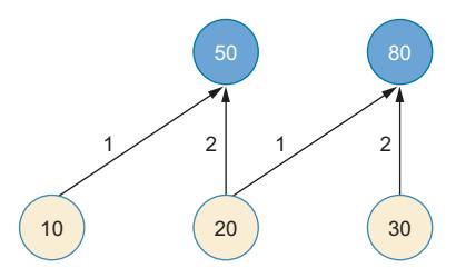
Figure 2.26 A simple causal convolution for the values 10, 20, 30 with a kernel with weights of 1, 2. The number 50 after convolution only depends on the past and present values (10, 20) but not on the future value of 30.

You see in figure 2.26 that the second (upper) layer has fewer elements. To make all layers the same size, a zero padding is added to the beginning of the input layer. In that case, figure 2.26 becomes figure 2.27.

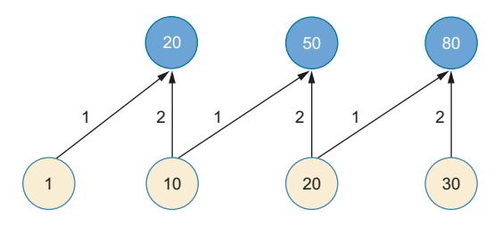
Figure 2.27 A simple causal convolution for the values 10, 20, 30 and the kernel 1, 2 with 0 padding

HANDS-ON TIME If you want to get a better understanding how 1D convolution works, you can go through the notebook http://mng.bz/5aBO. In this notebook, we also introduce time-dilated causal convolution, allowing for long-range time dependencies.

Now you’ve seen the basic architectural building blocks used in DL: fully connected, convolutional, and recurrent NNs. These are just building blocks, and you can use these in combination with each other. For example, you could feed an image into a convolutional network, then use an RNN to produce ordered output as text. This combination has been successfully used to create captions for images.

But, so far, we’ve not shown you an important part—how to do the adaptation of the weights in networks. In the next chapter, we take a step back from NNs with millions of weights to training a linear regression with just one or two weights. It’s astonishing that all the architectures we discussed so far (from simple linear regression to advanced models like CNNs or time-dilated convolutional networks) can be trained with the same procedure: gradient descent.

Summary

• A fully connected neural network (fcNN) consists of stacked layers of neurons.
• In an fcNN, each neuron connects to each neuron of the previous layer.
• The input to a neuron is given by the weighted sum of the connected neurons in the previous layer.
• That weighted sum passed through an activation function computes the output of a neuron.
• The non-linearity of the activation function is essential because a stack of layers could otherwise be replaced by one layer.
• Use the relu activation function for hidden layers. It is known to yield a more efficient training, compared to the sigmoid activation function.
• Use softmax as an activation function in the output layer when doing classification. The output of the softmax function can be interpreted as probability for a certain class label.
• A convolutional neural network (CNN) consists of a convolutional part, where features are extracted from the input data, and a fully connected part, where the features are combined to the output of the CNN.
• The convolutional part of a CNN consists of stacked layers of feature maps.
• Each neuron in a feature map only connects to a small patch of the previous feature map. This reflects the local structure of image data.
• The high performance of deep NNs relies on the fact that they learn a hierarchy of optimal features for the given task.
• NNs work best when the NN architecture exploits a known structure of the data so that these don’t have to learn it from scratch. Therefore,
• If your data comes from images (or has other 2D structures), use 2D CNNs to exploit the local structure of images by local connections and shared weights.
• If your data comes from sequences, use 1D convolutions if possible; otherwise, use recurrent NNs.
• If you have no particular structure, use fcNNs.

Principles of curve fitting

This chapter covers

• How to fit a parametric model
• What a loss function is and how to use it
• Linear regression, the mother of all neural networks
• Gradient descent as a tool to optimize a loss function
• Implementing gradient descent with different frameworks

DL models became famous because they outperformed traditional machine learning (ML) methods in a broad variety of relevant tasks such as computer vision and natural language processing. From the previous chapter, you already know that a critical success factor of DL models is their deep hierarchical architecture. DL models have millions of tunable parameters, and you might wonder how to tune these so that the models behave optimally. The solution is astonishingly simple. It’s already used in many methods in traditional ML: you first define a loss function that describes how badly a model performs on the training data and then tune the parameters of the model to minimize the loss. This procedure is called fitting.

In ML models that have simple loss functions, it’s often possible to provide a formula that lets you compute the optimal parameter values from the data. Yet, this isn’t the case for complex models. For complex models, it took several decades to develop sophisticated optimization procedures. DL almost exclusively uses an approach to determine the parameters: this is called gradient descent. In this chapter, you’ll see that gradient descent is an astonishingly simple technique. It’s still kind of a miracle that this technique works so well in DL, while more advanced procedures for optimization fail.

All the components needed for DL—a model with weights and a loss function used to fit the weights to the (training) data—are already present in much simpler models like linear regression. In order to give you a clear picture of the gradient descent method, we demonstrate step by step how it works for fitting a simple linear regression model. This, in fact, is the smallest neural network (NN) possible. We introduce the loss function, which is most often used to fit a linear regression model, and show how to determine the parameter values that minimize this loss function. Think of linear regression as the “hello world” of machine and deep learning. Let’s have a look at linear regression through the eyes of DL.

3.1 “Hello world” in curve fitting

Let’s look at a simple model in the form of linear regression. Imagine you’re a novice medical assistant, and you work together with a gynecologist who asks you to notify her if a patient shows an unusual systolic blood pressure (SBP) during routine checks. For this purpose, she provides you with a table that shows a normal range of SBP values for each age category. According to this table, it’s normal that the SBP increases with age. This raises your curiosity. You wonder whether the data is consistent with actual data measured during past routine checks. To follow up on this, you want to look at some other data. Fortunately, you’re allowed to use the data from your patients for internal analysis.

As a first step, you randomly select a set of 33 patients, who during at least one visit were diagnosed as healthy by the doctor. From each of the selected patients, you note information on age and blood pressure recorded during one of the routine checks, where the patient was diagnosed as healthy. To get an impression of the data, you can produce a scatter plot where you graph the SBP value versus the age (see figure 3.1).

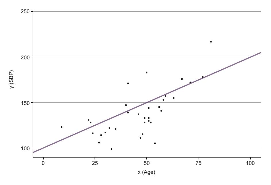
Figure 3.1 Scatter plot showing the systolic blood pressure (SBP) versus age (for women)

From figure 3.1, you can see that most SBP values are in the range 100 to 220. The scatter plot reveals that, similar to the table your boss gave you, there is indeed a trend indicating that for healthy women, blood pressure increases with age. It also makes sense that the table gives a range of normal blood pressures for each age because the relationship between age and SBP is far from deterministic. (Two healthy women with similar ages can have quite different blood pressure values.) Information in the table thus seems consistent with your observations.

The Simple Linear Model

You now want to go a step further and look for a model that describes how the blood pressure depends on age. Independent from individual variations in blood pressure, it seems that, on average, the SBP values somehow increase linearly with the age of the women. You can manually draw a straight line through the points to end up with something similar to the line in figure 3.1. We can describe such a straight line by the linear model

$$y = a cdot x + b$$

where a represents the slope of the line and b is the intercept with the y-axis. Another way (which is more DL-like) is to look at the model of the graph shown in figure 3.2.

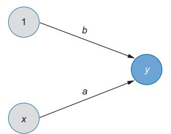
{alt=”Figure 3.2: Linear regression model (y = a · x + b) represented as a fully connected neural network (fcNN) or a computational graph, illustrating input x, parameters a and b, and the computation of output y.”}

This graph is probably the smallest fully connected network (fcNN) you can think of. At the same time, it’s a part of the more complicated one that was shown in figure 1.2 in chapter 1. Moreover, it graphically represents the computational steps that you need to take to compute a value for y when you have a value for x and you know the parameter values a and b:

• Take x and multiply it by a
• Take 1 and multiply it by b
• Add both results to get

Regardless of whether you interpret the model as a line equation or as an fcNN, you can only use the model to compute an estimate for the mean y based on a given value of x when the values for a and b are fixed. Therefore, a and b are called the parameters of the model. Because the parameters enter the model linearly, we call the model a linear model, and because there’s only one input feature x, we call it a simple linear model. How can you get appropriate values for the parameters a (slope) and b (intercept) of the linear model that best describes the data?