Smartphone-Based Real-Time Digital Signal Processing

Second Edition

Nasser Kehtarnavaz, Abhishek Sehgal, and Shane Parris
University of Texas at Dallas

Synthesis Lectures on Signal Processing

Editor: José Moura, Carnegie Mellon University

Synthesis Lectures in Signal Processing publishes 80- to 150-page books on topics of interest to signal processing engineers and researchers. The Lectures exploit in detail a focused topic. They can be at different levels of exposition—from a basic introductory tutorial to an advanced monograph—depending on the subject and the goals of the author. Over time, the Lectures will provide a comprehensive treatment of signal processing. Because of its format, the Lectures will also provide current coverage of signal processing, and existing Lectures will be updated by authors when justified.

Lectures in Signal Processing are open to all relevant areas in signal processing. They will cover theory and theoretical methods, algorithms, performance analysis, and applications. Some Lectures will provide a new look at a well established area or problem, while others will venture into a brand new topic in signal processing. By careful reviewing the manuscripts we will strive for quality both in the Lectures’ contents and exposition.

Books in Series

Anywhere-Anytime Signals and Systems Laboratory: From MATLAB to Smartphones, Second Edition

Nasser Kehtarnavaz, Fatemeh Saki, and Adrian Duran 2018

Anywhere-Anytime Signals and Systems Laboratory: From MATLAB to Smartphones

Nasser Kehtarnavaz and Fatemeh Saki 2016

Smartphone-Based Real-Time Digital Signal Processing

Nasser Kehtarnavaz, Shane Parris, and Abhishek Sehgal 2015

An Introduction to Kalman Filtering with MATLAB Examples

Narayan Kovvali, Mahesh Banavar, and Andreas Spanias 2013

Sequential Monte Carlo Methods for Nonlinear Discrete-Time Filtering

Marcelo G.S. Bruno 2013

Processing of Seismic Reflection Data Using MATLAB™

Wail A. Mousa and Abdullatif A. Al-Shuhail 2011

Fixed-Point Signal Processing

Wayne T. Padgett and David V. Anderson 2009

Advanced Radar Detection Schemes Under Mismatched Signal Models

Francesco Bandiera, Danilo Orlando, and Giuseppe Ricci 2009

DSP for MATLAB™ and LabVIEW™ IV: LMS Adaptive Filtering

Forester W. Isen 2009

DSP for MATLAB™ and LabVIEW™ III: Digital Filter Design

Forester W. Isen 2008

DSP for MATLAB™ and LabVIEW™ II: Discrete Frequency Transforms

Forester W. Isen 2008

DSP for MATLAB™ and LabVIEW™ I: Fundamentals of Discrete Signal Processing

Forester W. Isen 2008

The Theory of Linear Prediction

P. P. Vaidyanathan 2007

Nonlinear Source Separation

Luis B. Almeida 2006

Spectral Analysis of Signals: The Missing Data Case

Yanwei Wang, Jian Li, and Petre Stoica 2006

www.morganclaypool.com

DOI 10.2200/S00885ED2V01Y201811SPR016

A Publication in the Morgan & Claypool Publishers series SYNTHESIS LECTURES ON SIGNAL PROCESSING

Lecture #16

Series Editor: José Moura, Carnegie Mellon University

Series ISSN
Print 1932-1236 Electronic 1932-1694

ABSTRACT

Real-time or applied digital signal processing courses are offered as follow-ups to conventional or theory-oriented digital signal processing courses in many engineering programs for the purpose of teaching students the technical know-how for putting signal processing algorithms or theory into practical use. These courses normally involve access to a teaching laboratory that is equipped with hardware boards, in particular DSP boards, together with their supporting software. A number of textbooks have been written discussing how to achieve real-time implementation on these hardware boards. This book discusses how to use smartphones as hardware boards for real-time implementation of signal processing algorithms as an alternative to the hardware boards that are used in signal processing laboratory courses. The fact that mobile devices, in particular smartphones, have become powerful processing platforms led to the development of this book enabling students to use their own smartphones to run signal processing algorithms in real-time considering that these days nearly all students possess smartphones. Changing the hardware platforms that are currently used in applied or real-time signal processing courses to smartphones creates a truly mobile laboratory experience or environment for students. In addition, it relieves the cost burden associated with using dedicated signal processing boards noting that the software development tools for smartphones are free of charge and are well-maintained by smartphone manufacturers. This book is written in such a way that it can be used as a textbook for real-time or applied digital signal processing courses offered at many universities. Ten lab experiments that are commonly encountered in such courses are covered in the book. This book is written primarily for those who are already familiar with signal processing concepts and are interested in their real-time and practical aspects. Similar to existing real-time courses, knowledge of C programming is assumed. This book can also be used as a self-study guide for those who wish to become familiar with signal processing app development on either Android or iPhone smartphones. A zipped file of the codes discussed in the book can be acquired from this third-party website http://sites.fastspring.com/bookcodes/product/SignalProcessingBookcodesSecondEdition.

KEYWORDS

smartphone-based signal processing, real-time signal processing using smartphones, smartphones as signal processing boards

Introduction

Smartphone Implementation Tools

Smartphone Implementation Shells

Android Implementation

iPhone Implementation

Overview of ARM Processor Architecture

Data Flow and Registers

Organization of Chapters

Software Package of Lab Codes

References

Android Software Development Tools

Installation Steps

Java JDK

Android Studio Bundle and Native Development Kit

Environment Variable Configuration

Android Studio Configuration

Android Emulator Configuration

Android Studio Setup for Mac

LAB 1: Getting Familiar with Android Software Tools

Lab Exercise

iOS Software Development Tools

App Development

Setting-up App Environment

Creating Layout

Implementing C Codes

Executing C Codes Via Objective-C

Swift Programming Language

LAB 2: iPhone App Debugging

Lab Exercise

Analog-to-Digital Signal Conversion

Sampling

Quantization

References

LAB 3: Android Audio Signal Sampling

Demo Application

Application Code

Recording

Processing.Java

JNI Native C Code

Superpowered SDK

Multi-Threading

Multi-Rate Signal Processing

Lab Exercises

LAB 4: iPhone Audio Signal Sampling

App Source Code

App Code Discussion

Recording

Native C Code

Multi-Threading

Multi-Rate Signal Processing

Lab Exercises

Fixed-Point vs. Floating-Point

Q-Format Number Representation

Floating-Point Number Representation

Overflow and Scaling

Some Useful Arithmetic Operations

Division

Sine and Cosine

5.4.3 Square-Root

LAB 5: Fixed-Point and Floating-Point Operations

L5.1 App Structure

L5.2 NEON SIMD Coprocessor

L5.3 Lab Exercises

5.6 References

6 Real-Time Filtering

6.1 FIR Filter Implementation

6.2 Circular Buffering

6.3 Frame Processing

6.4 Finite Word Length Effect

6.5 References

LAB 6: Real-Time FIR Filtering, Quantization Effect, and Overflow

L6.1 Filter Design

L6.2 ARM Overflow Detection

L6.3 Lab Exercises

7 Adaptive Filtering

7.1 Infinite Impulse Response Filters

7.2 Adaptive Filtering

7.3 References

LAB 7: IIR Filtering and Adaptive FIR Filtering

L7.1 IIR Filter Design

L7.2 Adaptive FIR Filter

L7.3 Lab Exercises

8 Frequency Domain Transforms

8.1 Fourier Transforms

8.1.1 Discrete Fourier Transform

8.1.2 Fast Fourier Transform

8.2 Leakage

8.3 Windowing

8.4 Overlap Processing

8.5 Reconstruction

8.5.1 Inverse Fourier Transform

8.5.2 Overlap-Add Reconstruction

8.6 References

LAB 8: Frequency Domain Transforms–DFT and FFT

L8.1 Lab Exercises

9 Code Optimization

9.1 Code Timing

9.2 Linear Convolution

9.3 Compiler Options

9.4 Efficient C Code Writing

9.5 Architecture-Specific Optimizations

9.5.1 Target Architecture

9.5.2 ARM Hardware Capabilities

9.5.3 NEON Intrinsics

LAB 9: Code Optimization

L9.1 Compiler Options

L9.2 Target Architecture (Android Only)

L9.3 Code Modification

9.7 References

10 Implementation Via Matlab Coder

10.1 Matlab Function Design

10.2 Test Bench

10.3 Code Generation

10.4 Source Code Integration

10.5 Summary

10.6 References

LAB 10: Matlab Coder Implementation

L10.1 Lab Exercises

Authors’ Biographies

Index

Preface

Real-time or applied digital signal processing courses are offered as follow-up courses to conventional or theory-oriented digital signal processing courses in many electrical engineering curricula. The purpose of offering real-time or applied digital signal processing courses is to enable students to bridge the gap between signal processing theory and implementation aspects.

A typical real-time or applied digital signal processing course is normally held within the confines of a teaching laboratory room that is equipped with implementation hardware platforms and the accompanying software for those platforms. The fact that mobile devices, in particular smartphones, have become powerful processing platforms led to the development of this book toward enabling students to use their own smartphones as implementation platforms for running signal processing algorithms as apps considering that these days nearly all students possess smartphones. Changing the hardware platforms that are normally used in real-time applied signal processing courses to smartphones creates a truly mobile laboratory experience or environment for students. In addition, it relieves the cost burden associated with using dedicated signal processing hardware boards noting that the software development tools for smartphones are free of charge and are well-maintained by smartphone manufacturers.

This book is written in such a way that it can be used as a textbook for real-time or applied digital signal processing courses offered at many universities. Ten lab experiments that are commonly encountered in such courses are covered in the book. This book is written primarily for those who are already familiar with signal processing concepts and are interested in their real-time and practical aspects. Similar to existing real-time courses, knowledge of C programming is assumed. This book can also be used as a self-study guide for those who wish to become familiar with signal processing app development on either Android or iPhone smartphones. In this second edition, various updates are made to reflect the newer versions of the software tools used in the first edition.

The smartphone-based approach covered in this book eases the constraint of a dedicated signal processing laboratory for the purpose of offering applied or real-time signal processing courses as it provides a truly mobile platform for implementation of signal processing algorithms. A zipped file of the codes discussed in the book can be acquired from this third-party website http://sites.fastspring.com/bookcodes/product/SignalProcessingBookcodesSecondEdition.

As a final note, I would like to thank my co-authors and ex-students, Abhishek Sehgal and Shane Parris, for their contributions, in particular for the development of the lab codes, in the first and second editions of this book.

Nasser Kehtarnavaz November 2018

Introduction

Applied or real-time digital signal processing courses offered at many universities have greatly enhanced students’ learning of signal processing concepts by covering practical aspects of implementing signal processing algorithms. DSP processor boards are often deployed in these courses. To a lesser extent, ARM-based boards such as Raspberry Pi[1] are utilized. A number of textbooks are available discussing how to implement signal processing algorithms on DSP boards, e.g., [2–6]. This book is written to provide an alternative hardware platform which students can use in a truly mobile manner and at no cost as it is already in their possession, that being their own smartphones.

Not only do there exist hardware and software costs associated with equipping a teaching laboratory with DSP or other types of signal processing boards, in many cases these boards are confined to a specific teaching laboratory location. Taking advantage of the ubiquitous utilization of ARM processors in mobile devices, in particular smartphones, this book covers an alternative approach to teaching applied or real-time DSP courses by enabling students to use their own smartphones to implement signal processing algorithms. Changing the hardware platforms that are currently used in applied or real-time signal processing courses to smartphones creates a truly mobile laboratory experience or environment for students. In addition, it relieves the cost burden associated with using a dedicated signal processing board noting that the software development tools for smartphones are free of charge and are well-maintained.

This book addresses the process of developing signal processing apps on smartphones in a step by step manner. It shows how to acquire sensor data, implement typical signal processing algorithms encountered in a real-time or applied digital signal processing course, and how to generate output or display information. It should be noted that these steps are carried out for both the Android and iOS operating systems and besides smartphones, the apps developed can be run on any ARM-based mobile targets such as tablets. The laboratory experiments that are included cover the following topics: signal sampling and i/o buffering, quantization effects, fixed-point vs. floating-point implementation, FIR filtering, IIR filtering, adaptive filtering, DFT/FFT frequency transformation, and optimization techniques to gain computational efficiency.

1.1 Smartphone Implementation Tools

The main challenge in this alternative approach to real-time or applied digital signal processing courses lies in the difference between the programming environments on smartphones and

C programming normally used in such real-time courses. Since a typical applied or real-time signal processing course requires familiarity with C programming, the same C programming familiarity is retained for this alternative approach, i.e., by not requiring students to know other programming languages. This challenge is met here by developing a Java (for Android smartphones) and an Objective-C (for iPhone smartphones) software shell to run C codes seamlessly so that the prerequisite programming knowledge students need to have would be no different than what is currently required.

To allow C codes to be written and compiled on Android smartphone targets, the following cost-free downloadable development tools are utilized: Android Studio Bundle (Studio Bundle) [[7]] and Android Native Development Kit (NDK) [[8]]. The Studio Bundle provides a comprehensive development environment incorporating the IntelliJ IDEA Integrated Development Environment (IDE), Android SDK plug-ins, and an emulator. The NDK provides the support for incorporating C/C++ codes within Android Studio.

To allow C codes to be written and compiled on iOS smartphone targets (iPhones), the Xcode IDE [[9]] and a Mac computer running OS X are utilized. It is worth stating that for iPhone implementation, it is required to register as an iOS developer to be able to run iPhone apps [[10]]. The Xcode IDE incorporates an editor, the iOS SDK, a built-in debugger for C, and an iPhone/iPad simulator.

1.2 SMARTPHONE IMPLEMENTATION SHELLS

The developed implementation shells for the Android and iPhone platforms provide the programming environment needed to perform signal processing laboratory experiments. As shown in Figure [1.1], the shells comprise parts or components which match in functionality for the two platforms. The major difference between the two platforms lies in the programming language. For Android smartphones, the programming language of the shell is Java, and for iPhone smartphones, it is Objective-C. Both platforms support implementing codes written in C and this feature is used to provide a uniform programming approach regardless of the type of smartphones students possess.

1.2.1 ANDROID IMPLEMENTATION

The Android shell consists of the following three major parts or components.

User Interface The UI comprises the so-called main activity in Java which allows controlling the shell operation and displaying outputs. The component PreferencesUI complements the main activity by controlling operational parameters.

I/O Handler The audio I/O is split into three modules depending on their functionality. Microphone recording is handled by the module WaveRecorder, audio file reading is handled by the module WaveReader, and speaker and debug outputs are handled by the module WaveSaver. The user is given the option to select one of the two modules WaveRecorder and WaveReader. In both cases, the module WaveRecorder is used for outputs.

Processing This module allows running C codes within the Android shell. Additional code segments are written to interface with the Java modules using the Java Native Interface (JNI) programming framework.

1.2.2 IPHONE IMPLEMENTATION

The iPhone shell also consists of three major parts that match the Android shell.

User Interface (UI) The UI module handles displaying program outputs and all interactions with the user. It provides an interface for the user to change the parameters required by the processing algorithm. The component Main.Storyboard contains the UI elements and the component ViewController handles all UI events such as user interaction or parameter changes.

I/O Handler This module gathers data to be processed by the processing algorithm depending on the source specified by the user. The component IosAudioController described in [[11]] is used to gather data from the microphone and provide data to a C code for processing. This component is also responsible for outputting processed audio signals to the speaker. When using an audio file, the component audioReader handles reading stored audio files and passing them to C codes for processing.

Processing This module allows running signal processing algorithms for the lab experiments that are written in C. This module processes and returns data provided by the I/O Handler.

1.3 OVERVIEW OF ARM PROCESSOR ARCHITECTURE

ARM (Advanced RISC Machine) is the processing engine that is used in modern smartphones. The ARM architecture has been extensively used in embedded systems. Its designs are licensed and incorporated into a wide range of embedded systems and low power mobile devices. The ARM architecture refers to a family of reduced instruction set computing (RISC) architectures produced by the company ARM. The most common architectures currently in use for mobile devices are the ARMv7 architecture which supports 32-bit addressing/arithmetic and the ARMv8 architecture which supports 64-bit addressing/arithmetic. An overview of the ARMv7 architecture is provided next.

1.3.1 DATA FLOW AND REGISTERS

The RISC nature of the ARM architecture means that arithmetic operations take place in a load/store manner. Figure [1.2] shows a diagram of the dataflow in an ARM core. ARM registers, that are all of uniform 32-bit width, consist of 13 general purpose registers (r0 to r12) and these 3 additional special use registers: stack pointer (SP or r13) which contains a pointer to the active stack, link register (LR or r14) which stores a return value when a branch instruction is called, and program counter (PC or r15) which contains a pointer to the current instruction being executed. In addition, there is one special register called Current Program Status Register (CPSR) which holds Application Program Status Register (APSR) and additional processor state flags. APSR refers to the ALU status flag bits set by the previous instruction in bits 31 to 27 of CPSR. Starting with bit 31, these values indicate negative, zero, carry, overflow, and saturation.

The execution pipeline varies between different versions of the ARM architecture. Instructions can be either from the ARM instruction set, which consists of 32-bit instructions, or from the Thumb instruction set, which consists of 16-bit instructions providing a compact data processing capability.

Some other features of the ARM architecture include barrel shifter, shown as part of the ALU in Figure [1.3], which is capable of performing logical left and right shifts, arithmetic right shifts, rotate right, and rotate right extended operations on operand B. Another feature is the ability to perform conditional execution. For instance, when decrementing an index as part of a loop, the test for zero can be performed with no overhead as part of the subtraction operation; the condition result is then used to break out of the loop. Other features such as the Advanced SIMD (NEON) coprocessor [[12]] will be discussed in later chapters. Interested readers can refer to [[13]] for additional and more detailed materials regarding the ARM architecture.

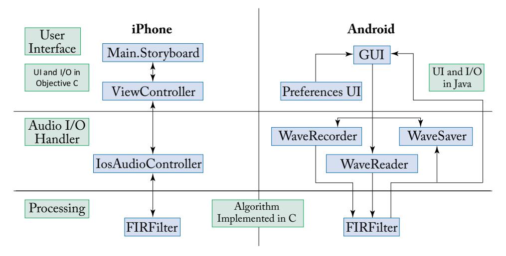
Figure 1.1: Components of the developed shell programs to run C codes on iPhone and Android smartphones.

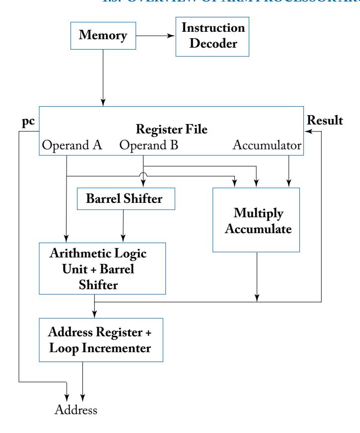
Figure 1.2: ARM processor data flow.

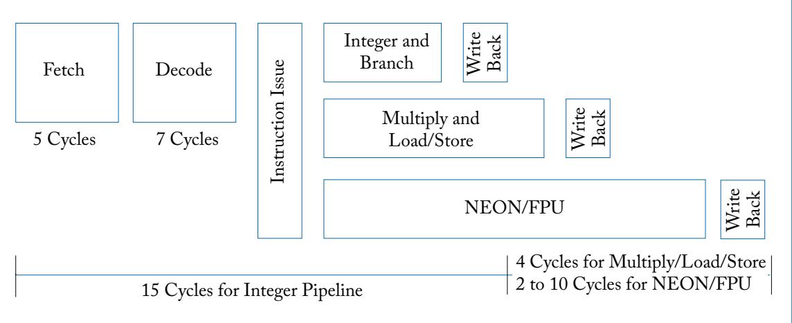
Figure 1.3: ARM Cortex-A15 instruction pipeline.

1.4 ORGANIZATION OF CHAPTERS

The chapters that follow are organized as follows. In Chapters [2] and [3], the smartphone software tools are presented, and the steps one needs to take in order to create a basic smartphone app are discussed. Chapter [2] covers the setup of the Android Studio programming environment, and Lab [L1] shows the development of a “Hello World” app for Android smartphones.

Chapter [3] and Lab [L2] are the counterparts of Chapter [2] and Lab [L1] focusing instead on the iOS operating system. Chapter [3] details the setup of the Xcode programming environment and duplicates the “Hello World” app from Lab [L1]. It also includes the debugging tool for iOS smartphones.

Chapter [4] introduces the topics of signal sampling and frame-based processing, and the steps that are required to interface with the A/D and D/A (analog-to-digital and digital-toanalog) converters for audio signal input and output on a smartphone target. As part of this process, the smartphone app shells for the Android and iOS smartphone platforms are covered in detail. The Java and Objective-C shells are discussed, and the steps to incorporate C codes are explained.

Labs [L3] and [L4] in Chapter [4] show how to sample an analog signal, process it, and produce an output in real-time on an Android and iOS smartphone target, respectively. Lab [L3] covers the Android development environment, and Lab [L4] the iOS development environment. These lab experiments involve processing a frame of signal samples captured by the smartphone microphone. The frame length can be altered by the user through a graphical-user-interface (GUI) settings menu. The sampling rate can also be altered depending on the sampling rates permitted by the A/D converter of the smartphone target used. It is normally possible to alter the sampling rate on a smartphone from 8–48 kHz. A low-pass FIR filter together with a user specified delay are considered in this lab experiment. The delay is meant to simulate an additional signal processing algorithm running on the ARM processor of the smartphone. The delay can be changed by the user through the settings menu, adding additional processing time to the low-pass filtering time. By increasing the sampling frequency or lowering the sampling time interval, data frames will get skipped and hence a real-time throughput cannot be met. Besides skipped frames noted on the GUI, one can hear both the original signal and the filtered signal through the speaker of the smartphone and notice the distortion caused by skipped frames due to the real-time demand. Distortion can also be experienced by increasing the processing time delay, thus demonstrating that a real-time throughput is a balance between computational complexity and computation rate. Processing of one frame of data needs to be done in less than N dt sec in order to achieve a real-time throughput, where N denotes the frame length and dt the sampling time interval. For example, for a sampling rate of 8 kHz and a frame length of 256, the processing needs to be completed within 32 ms in order for all the frames to get processed without any frames getting skipped.

In Chapter [5], fixed-point and floating-point number representations are discussed and their differences are pointed out. Lab [L5] in Chapter [5] gives suggestions on how one may cope

with the overflow problem. This lab experiment involves running an FIR filter on a smartphone using fixed-point arithmetic. 16 bits are used to quantize the double precision floating-point filter coefficients generated by a filter design package. Due to quantization, the frequency response of the filter is affected. The quantization word length can be adjusted in the settings menu and the deviation of the frequency response magnitude can be observed in a graph displayed automatically in the user interface. The settings menu allows the user to alter the quantization bits to examine the deviation of the frequency response from the frequency response of the floating-point implementation. In addition, due to quantization, overflows may occur depending on the number of coefficients. This experiment shows how scaling can be used to overcome overflows by scaling down input samples and scaling back up output samples generated by the filter.

Chapters [6] and [7] discuss common filters used in digital signal processing applications. Lab [L6] in Chapter [6] covers FIR (finite impulse response) filtering and Lab [L7] in Chapter [7] shows how adaptive filtering can be used to perform system identification. The experiment in Lab [L7] exhibits adaptive filtering where an adaptive FIR filter based on the least mean squares (LMS) coefficient update is implemented to match the output of an IIR (infinite impulse response) filter. The error between the output of the adaptive FIR filter and the IIR filter for an input signal is measured and displayed on the smartphone screen in real-time as the app runs. Over time the error between the two outputs converges toward zero. The user can experiment with the rate of convergence by altering the adaptive filter order through the settings menu without needing to recompile the code. As the filter order is increased, it can be observed that the convergence rate also increases. The drawback of increasing the filter order, that is an increase in the processing time, can also be observed. This experiment allows one to see how a tradeoff between convergence rate and real-time throughput can be established.

Chapter [8] covers frequency domain transforms and their implementation using frame-based processing. Lab [L8] explores the computational complexity of Fourier transform algorithms and shows the utilization of Fourier transform for solving linear systems. The first part of this lab experiment compares the computational complexity of discrete Fourier transform (DFT) and fast Fourier transform (FFT) by first computing the DFT directly, having the computational complexity of O(N^2), and then via FFT, having the computational complexity of O(N log N). In the second part of this lab, a filter is implemented in the frequency domain by using Fourier transform three times. Frequency domain filtering is done by complex multiplication between two transformed signals. This approach is observed to be more computationally efficient than convolution when the length of the filter is made long.

Code efficiency issues are addressed in Chapter [9], in which optimization techniques, as well as the use of intrinsics to access hardware features of the ARM processor, are discussed. Lab [L9] in this chapter provides a walkthrough of optimization techniques and their impact on a signal processing app. In this lab experiment, the steps one can take to speed up code execution on a smartphone target are covered. These steps include changing compiler settings, writing efficient C code, and using architecture-specific functions for the ARM processor. The

1. INTRODUCTION

FIR filtering (linear convolution) code is used here to show the effects of these steps on the real-time throughput. Compiler options constitute the simplest but an effective optimization step. By changing these options, the compiler produces executable binaries that are either optimized for higher processing speed or for lower memory footprint. After carrying out various compiler optimization options and observing the computational efficiency gains, one can take advantage of the NEON SIMD coprocessor that modern smartphones possess to perform vector data processing. One method of using the NEON coprocessor is the use of NEON intrinsics within C codes. These intrinsics allow access to architecture specific operations such as fused multiply-accumulate, the Newton–Raphson method for division and square root, data format conversions, and saturating arithmetic operations. In other words, many of the architecture specific features of the ARM processor can be accessed by utilizing intrinsic functions within C codes. The initial processing algorithms can be used as a basis for deciding where to utilize intrinsics. In this lab, it is demonstrated that the convolution of two signal sequences can be performed more efficiently by utilizing a vectorized loop via NEON intrinsics.

Chapter [10] presents an optional alternative approach using the MATLAB Coder [14] from the company MathWorks that can be used to rapidly take a signal processing algorithm implemented in MATLAB and transfer it to a smartphone target. The lab experiment (Lab [L10]) covered in the chapter exhibits the setup process for the MATLAB Coder tool provided by MathWorks which allows converting MATLAB functions into C functions. This requires the use of MATLAB version 2016a with the MATLAB Coder included. The experiment discussed in this chapter shows how to convert a MATLAB function into a C function and implement it into an Android or an iOS app.

1.5 Software Package of Lab Codes

For performing the laboratory experiments, similar to existing real-time or applied digital signal processing courses, familiarity with C programming and MATLAB are assumed. The lab codes can be obtained from the third-party link http://sites.fastspring.com/bookcodes/product/SignalProcessingBookcodesSecondEdition. The lab subfolders found under Android and iOS in the package include all the codes necessary to implement the labs. For the iOS platform, the necessary software is the Xcode IDE which may be installed from the Mac App Store free of charge. In order to deploy and test apps on an iOS device, note that it is first required to enroll in the iOS Developer Program. The shell for the iOS operating system is included as part of the above package so that all the codes can be acquired together in one place.

In the absence of a smartphone target, the simulator can be used to verify code functionality by using data already stored in a data file or from sensors present on the host machine running the simulator. However, when using the simulator, sensor support is often limited and performance is not comparable to that of an actual smartphone target. To be able to process signals in real-time, an actual smartphone target is needed. All the hardware necessary to run the laboratory experiments covered in this book is available on a modern smartphone.

1.6 REFERENCES

• [1] https://www.raspberrypi.org/

The Android development environment used here is the IntelliJ IDEA-based Android Studio Bundle (Android Studio). C codes are made available to the Android Java environment through the use of the Java Native Interface (JNI) wrapper. Thus, it is also necessary to install the Android Native Development Kit (NDK). This development kit allows one to write C codes, compile, and debug them on an emulated Android platform or on an actual Android smartphone/tablet.

Screenshots are used to show the steps and configuration options involved in the installation when using the Windows operating system. The same software tools are also available for other operating systems.

2.1 Installation Steps

Start by creating a directory where the tools are to be installed. A generic directory of C:Android is used here and the setup is done such that all Android development related files are placed within the C:Android directory.

2.1.1 Java JDK

If the Java Development Kit (JDK) is not already installed on your computer or you do not have the latest version, download it from Oracle’s website and follow the installation steps indicated by the installer. The latest JDK package at the time of this writing can be found on Oracle’s website at:

http://www.oracle.com/technetwork/java/javase/downloads/index.html

Click on the JDK Download button in the Java Platform, Standard Edition section shown in Figure [2.1a], and you will be taken to the page shown in Figure [2.1b]. From the list of supported platforms, select the correct version for your operating system. For example, if you are running a 64-bit operating system, select the appropriate package.



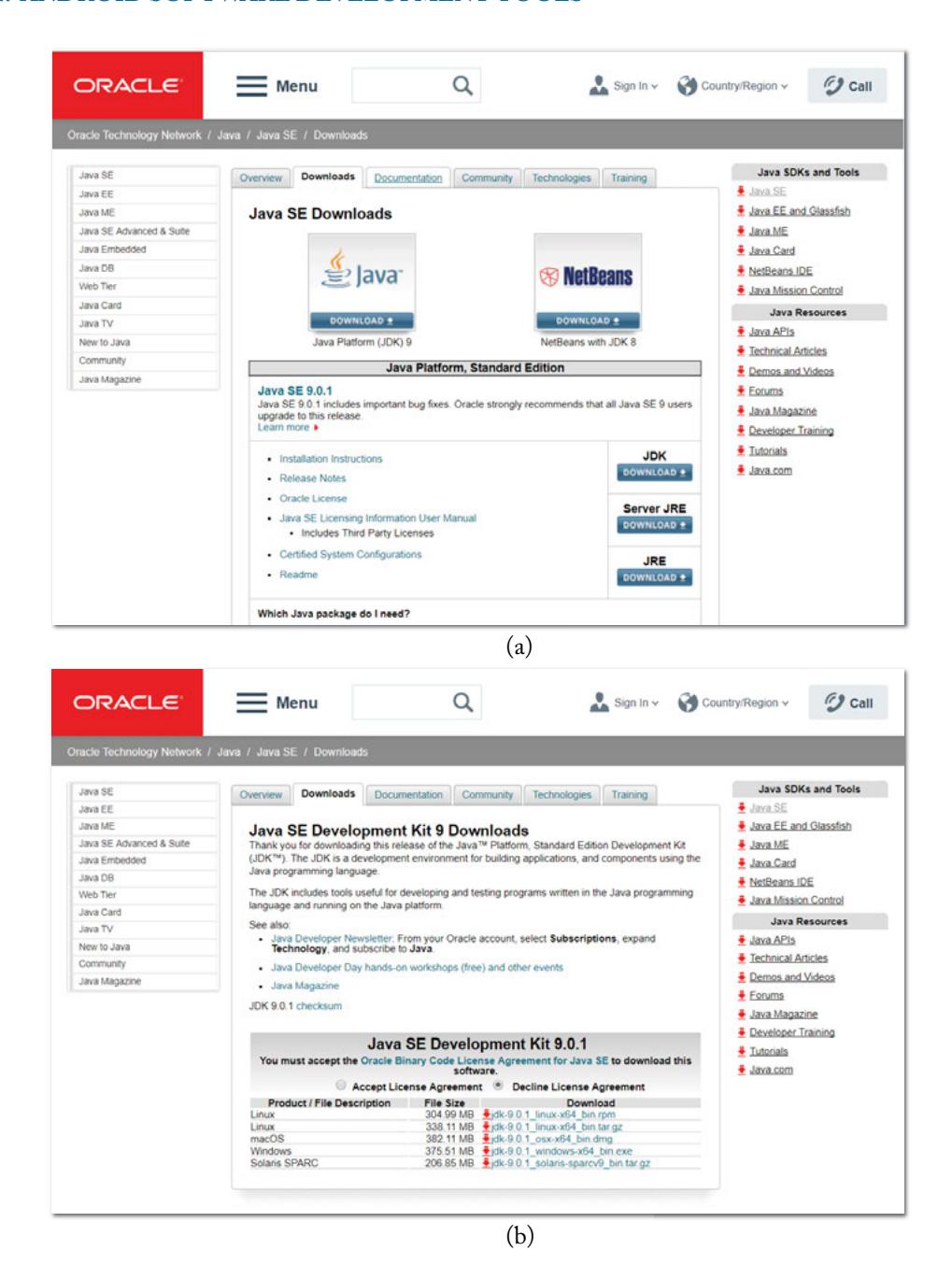
Figure 2.1: (a) Standard edition of Java platform; (b) Java downloads.

2.1.2 Android Studio Bundle and Native Development Kit

The most recent versions of Android Studio and the NDK at the time of this writing are used to run the lab experiments in the book. For the Windows installation, the Android Studio Bundle is available as an executable installer which incorporates the development environment. The SDK tools need to be installed separately from the development environment. In both cases, the installation binaries appear at this website, as depicted in Figure 2.2:

http://developer.android.com/sdk/index.html

Platform	SDK tools package	Size	SHA-256 checksum
Windows	sdk-tools-windows-3859397.zip	132 MB (138,449,982 bytes)	7f6037d3a7d6789b4fdc06ee7af041e071e9860c51f66f7a4eb5913df9871fd2
Mac	sdk-tools-darwin-3859397.zip	82 MB (86,182,133 bytes)	4a81754a760fce88cba74d69c364b05b31c53d57b26f9f82355c61d5fe4b9df9
Linux	sdk-tools-linux-3859397.zip	130 MB (136,964,098 bytes)	444e22ce8ca0f67353bda4b85175ed3731cae3ffa695ca18119cbacef1c1bea0

Figure 2.2: SDK packages.

The Android NDK is available in the form of a self-extracting archive at this website: http://developer.android.com/tools/sdk/ndk/index.html

Download the Android Studio, SDK, and NDK installation binaries into the Android directory created earlier and run the Android Studio installer.

During the installation of Android Studio, there are two important settings that are critical to do correctly; see Figures 2.3 and 2.4. For the setting shown in Figure 2.3, make sure that all the components are selected for installation, and for the setting shown in Figure 2.4, make sure that Android Studio is installed in the directory C:Android. The same procedure needs to be done for the Android SDK installation. To do so, manually create the directories by using the Browse option and create a Studio folder and a sdk folder. When the installer is finished, do not allow it to start Android Studio as additional configuration is still needed.

The last step is to extract the Android NDK to the folder C:Android by placing the archive executable in the folder and running it. When this action is completed, rename the folder android-ndk- to ndk.



Figure 2.3: Android Studio Setup.

2.1.3 Environment Variable Configuration

Before running Android Studio for the first time, the system environment needs to be set up by adding the SDK platform-tools folder to the system path variable and setting the variables to define the Android Virtual Device (AVD) storage location as well as the locations for the Android SDK and NDK. The steps listed here are for the Windows operating system. Similar steps need to be followed for other operating systems.

On your desktop, right click on the Computer icon and select Properties. Next, open the Advanced system settings menu and click on Environment Variables at the bottom of the Advanced tab; see Figure 2.5. Then, create new system variables by clicking the New… button below the System variables section, shown in Figure 2.6. There are three new system variables that need to be set: ANDROID_SDK_HOME with the value C:Android,



Figure 2.4: Configuration Settings.

ANDROID_SDK_ROOT with the value %ANDROID_SDK_HOME%sdk, and ANDROID_NDK_HOME with the value %ANDROID_SDK_HOME%ndk.

Then, add the following text to the end of your system path variable as shown in Figure 2.7;%ANDROID_SDK_ROOT%platform-tools. Be sure to include the semicolon which is used to separate the variables. Modifications are now complete and the settings menus can be closed.

2.1.4 Android Studio Configuration

Navigate to the C:AndroidStudiobin directory and edit the idea.properties file with a text editor. Uncomment the lines idea.config.path and idea.system.path and replace ${idea.home} with C:/Android for both of these lines. The final lines need to appear as



Figure 2.5: System Properties.



Figure 2.6: Environment Variables.

Figure 2.7: Edit System Variable.



Figure 2.8: idea.properties.

shown in Figure 2.8. At this time, also setup a shortcut to either studio.exe or studio64.exe on your desktop as this is the main executable for Android Studio.

Android Studio may now be started for the first time using the shortcut just created. The tool will prompt to import settings and check for the correct Java JDK. At the Install Type screen, select the Custom option and click Next. On the SDK Components Setup screen, verify that the Android SDK Location is properly detected as C:Androidsdk. If it is correct, click Finish

which will cause checking for any available updates to Android Studio. When this is done, the Android Studio home screen should appear as shown in Figure 2.9.



Figure 2.9: Android Studio.

Now run the SDK Manager, whose entry can be found by clicking on the Configure option. The SDK Manager will automatically select any components of the Android SDK which need updating, as illustrated in Figure 2.10. From this menu, additional system images for emulation and API packages for future Android versions can get added.

Click the Install option and allow the update process to complete.

2.1.5 Android Emulator Configuration

The last item to take care of is configuring an Android Virtual Device (AVD) on which the emulation and debugging are to be performed. From within the SDK Manager, open the Tools menu (see Figure 2.10) and select the Manage AVDs option to open the Android Virtual Device Manager as shown in Figure 2.11. By default, Android Studio creates an x86 AVD. Since our development focus is on ARM-based implementations, an ARM-based emulator instance is required. Begin by deleting any existing AVD instances.

1. Click the Create… button to start configuring the AVD (see Figure 2.12a).
2. Select the preferred device to use from the list. For the Device option, select a device with a good screen resolution for your computer—Nexus 5X is normally fine (see Figure 2.12b).



Figure 2.10: SDK tools.



Figure 2.11: Manage Android Virtual Device (AVD).



Figure 2.12: (a) AVDs; (b) AVD selection.

In the next page, a list of Android release versions appear. At the ABI column, Armeabi-v7a select ABI. If you are not able to see the option “Armeabi-v7a,” switch tab to “Other Images,” and download Lollipop Android 5.1 Armeabi-v7a.

For compatibility with smartphones released within the last two years, it is suggested to select the Target as the latest available version with the CPU/ABI as ARM (armeabi-v7a). You should now be able to create the AVD by clicking Finish. Select the AVD you just created in the list of devices (see Figure 2.13). Go to the AVD Manager from Tools, then select last column Action. Click Launch and wait for the AVD to boot (see Figure 2.14). Once the AVD launches, unlock the screen and get rid of the greeting message (see Figure 2.15). To run the Android emulator faster, Quick Boot can be used. Note that, for the first time, the emulator needs to be run using Cold Boot. By using Quick Boot for subsequent starts, the latest state is stored and used for future starts. This feature is set as default (see Figure 2.16).



Figure 2.13: AVD setting.



Figure 2.14: AVD booting.



Figure 2.15: AVD appearance.

2.1.6 Android Studio Setup for Mac

For Mac OS installation, the following softwares need to be installed: Xcode, Java Development Kit (JDK), Android Studio Development Bundle, and Android Native Development Kit (NDK). Xcode can be downloaded from the following link:

https://developer.apple.com/xcode/download/

Set the environment variable ANDROID_HOME to your Android SDK location. The correct syntax for setting your environment variable is:

export ANDROID_HOME=<path to SDK>/android/sdk

In order to find the SDK path, launch Android Studio and find the SDK location:

File > Project Structure > SDK Location: "Android SDK location"

The path for the SDK and platform tools directories is:

PATH: PATH=$PATH:$ANDROID_HOME/tools:$ANDROID_HOME/platform-tools

Once NDK is downloaded, set the NDK location to: home/dev folder (/dev).

It is worth noting that the Android NDK or SDK folders should not appear inside each other.

Set the ANDROID_NDK_HOME environment variable to the directory where the NDK is installed; for example:

export ANDROID_NDK_HOME=~/dev/android-ndk-r14b

Then the NDK directory should be added to PATH:

export PATH=$PATH:$ANDROID_NDK_HOME

The SDK is usually installed in the library. In order to find the folder, use cd ~/Library, and then open ~/Library/ in the terminal to find full path of SDK.

To check, write the following command in the terminal:

nano ~/.bash_profile

Then, in the nano ~/.bash_profile, write these commands (see Figure 2.17):

export ANDROID_HOME={YOUR_PATH}
export PATH=$PATH:$ANDROID_HOME/tools:$ANDROID_HOME/platform-tools
export ANDROID_NDK_HOME=[NDK_PATH]/android-ndk-[version]
export PATH=$PATH:$ANDROID_NDK_HOME

L1 Lab 1: Getting Familiar with Android Software Tools

This lab covers a simple app on the Android smartphone platform by constructing a “Hello world!” program. Android Studio and NDK tools are used for code development, emulation, and code debugging. All the codes needed for this and other labs can be extracted from the package mentioned in Chapter 1. Start by launching Android Studio, and if not already done, set up an Android Virtual Device (AVD) for use with the Android emulator.

• Begin by creating a new Android project using the Quick Start menu found on the Android Studio home screen.



Figure 2.17: Commands for bash profile setup.

• Set the Application Name to HelloWorld and the project location to a folder within the C:Android directory.
• Change the Company Domain to dsp.com so that the package name reads as com.dsp.helloworld. This is of importance later as it will affect the naming of your native code methods. Refer to Figure L1.1a for the previous three steps.
• The Target Android device should be set to Phone and Tablet using a Minimum SDK setting of API 15.
• Click Next and on the following screen choose to create a Blank Activity.
• Click Next again to create a Blank Activity and leave the default naming.
• Select Finish. The new app project is now created and the main app editor will open to show the GUI layout of the app.
• Navigate to the java directory of the app in the Project window and open the MainActivity.java file under com.dsp.helloworld, as shown in Figure L1.1b.



Figure L1.1: (a) Android Studio ‘Create New Project’ screen; (b) HelloWorld project structure in Android Studio.

The class that typically defines an Android app is called an Activity. Activities are generally used to define user interface elements. An Android app has activities containing various sections that the user might interact with such as the main app window. Activities can also be used to construct and display other activities—such as if a settings window is needed. Whenever an Android app is opened, the onCreate function or method is called. This method can be regarded as the “main” of an activity. Other methods may also be called during various portions of the app lifecycle as detailed at the following website:

http://developer.android.com/training/basics/activity-lifecycle/starting.html

In the default code created by the SDK, setContentView(R.layout.activity_main) exhibits the GUI. The layout is described in the file res/layout/activity_main.xml in the Package Explorer window. Open this file to preview the user interface. Layouts can be modified using the WYSIWYG editor which is built into Android Studio. For now the basic GUI suits our purposes with one minor modification detailed as follows.

• Open the XML text of the layout (see Figure L1.2) by double clicking on the Hello world! text or by clicking on the activity_main.xml tab next to the Graphical Layout tab.
• Add the line android:id="@+id/Log" within the <TextView/> section on a new line and save the changes. This gives a name to the TextView UI element.



Figure L1.2: XML text of the layout, showing the TextView section.

TextView in the GUI acts similar to a console window. It displays text. Additional text can be appended to it. By adding the android:id directive to TextView, it may be interfaced with in the app code.

After setting up the emulator and the app GUI, let us now cover interfacing with C codes. Note that it is not required to know the Java code syntax. The purpose is to show that the Java Native Interface (JNI) is a bridge between Java and C codes. Java is useful for handling Android APIs for sound and video i/o, whereas the signal processing codes are done in C. Of course, familiarity with C programming is assumed.

A string returned from a C code is considered here. The procedure to integrate native code consists of creating a C code segment and performing more alterations to the project. First, it is required to add support for the native C code to the project. The first step is to create a folder in which the C code will be stored. In the Project listing, navigate down to New > Folder > JNI to create a folder in the listing called jni. Refer to Figures L1.3–L1.6. Figure L1.5 shows how the Project listing view may be changed in order to show the jni folder in the main source listing.



Figure L1.3: Creating a JNI folder in Android Studio project.

Android Studio now needs to be configured to build a C code using the Gradle build system. Begin by specifying the NDK location in the project local.properties file according to Figure L1.7. Assuming the directory C:/Android is used for setting up the development tools, the location specification would be as follows:

ndk.dir=C:\Android\ndk



Figure L1.4: Specifying the JNI folder location.



Figure L1.5: Android Studio project listing showing the jni folder.



Figure L1.6: MainActivity.java file in Android Studio.



Figure L1.7: Configuring NDK location in local.properties.

Next, the native library specification needs to get added to the build.gradle file within the project listing, beneath the app section. This specification declares the name of the native library which is needed by Java to actually load the library, as well as the library target platform (e.g., armeabi, x86, mips). This is done by adding the following code to the defaultConfig section:

ndk {
        moduleName "HelloWorld"
        abiFilter "armeabi"
}

The correct placement of the code is shown in Figure L1.8.



Figure L1.8: Correct placement of NDK configuration in build.gradle.

The C code considered here consists of a simple method to return a string when it is called from the onCreate method. First, the code that defines the native method needs to be included. Create a new HelloWorld.c file. Add the following code and save the changes:

#import <jni.h>
jstring Java_com_dsp_helloworld_MainActivity_getString (
                             JNIEnv* env, jobject thiz )
{
     return (*env)->NewStringUTF(env, "Hello UTD!");
}

2. ANDROID SOFTWARE DEVELOPMENT TOOLS

This code defines a method that returns a Java string object according to the JNI specifications with the text “Hello UTD!”. The naming for this method is dependent on what is called fully qualified name of the native method which is defined in the MainActivity class. There are alternate methods of defining native methods that will be discussed in later labs.

It is important to note that due to a bug currently present in the Gradle build system, a dummy C source file needs to be created in the jni folder in order for the build process to complete successfully. Simply create a new source file, named dummy.c for example, without any code content.

Next, the native method needs to be declared within the MainActivity.java class (see Figure L1.9) according to the naming used in the C code. To do so, add this declaration below the onCreate method already defined:

public native String getString();

Now, add the following code within public class to load the native library:

static {
          System.loadLibrary("HelloWorld");
}

To use the TextView GUI object, it needs to be imported by adding the following declaration to the top of the MainActivity.java file:

import android.widget.TextView;

The TextView defined in the GUI layout needs to be hooked to the onCreate method by adding the following lines to the end of the onCreate method code section (after setContentView but inside the bracket):

TextView log = (TextView)findViewById(R.id.Log);
log.setText( getString() );

This will cause the text displayed in the TextView to be changed by the second line which calls the C getString method.

Save the changes and select the Make Project option (located under the Build category on the main toolbar). Android Studio would display the build progress and notify if any errors occur. Next, run the app on the Android emulator using the Run app option located in the Run menu of the toolbar. If an emulator is already running, an option will be given to deploy the app to the selected device (see Figure L1.10). Android Studio should launch the emulator and the screen (see Figure L1.11) would display “Hello UTD!”. To confirm that the display is being changed, comment out the line log.setText() and run the app again. This time the screen would display “Hello World!”



Figure L1.9: MainActivity class.

Note that the LogCat feature of Android Studio can be used to display a message from the C code. LogCat is equivalent to the main system log or display of the execution information. Here, the code from the previous project is modified to enable the log output capability as follows.

• Add the logging library to the build.gradle file (see Figure L1.8) by adding the line ldLibs "log" to the ndk section which was added previously.
• Add the Android logging import to the top of the HelloWorld.c source file (see Figure L1.12) by adding the line #include<android/log.h>.
• Add the following code to output the test message before the return statement:



Figure L1.10: Deployment target.



Figure L1.11: Emulator screen.

Figure L1.12: HelloWorld.c.

int classNum = 9001;
int secNum = 1;
__android_log_print(ANDROID_LOG_ERROR, "HelloWorld",
                    "DSP %d.%03d", classNum, secNum);

The __android_log_print() method (two underscores at the beginning) is similar to the printf function in C. The first two parameters are the log level and the message tag. The logging level is the priority of the message, the list of which can be found in the android/log.h header file. The tag is used to help identify the source of the message; in this case the name of the app. The next parameter is the message to be logged. For the above example, the string has the specified integer for the class number inserted, followed by the specified integer for the section number. The same number formatting that is possible when using the printf function may also be used here. For instance, the section number can be formatted to three characters width with leading zeros. Variables are last and are inserted with the formatting specified in the message string in the order they are listed.

Save the changes made to the HelloWorld.c source file and run the app again. This time, Android Studio should automatically open the Android DDMS window and show the LogCat screen. The message “DSP 9001.001” would appear in the listing if the previous procedures were performed properly (see Figure L1.13).



Figure L1.13: LogCat screen.

L1.1 LAB EXERCISE

Write a C function within the above Android shell to implement the following difference equation: y(n) = a * y(n-1) + x(n).

Let x(n) be a unit sample at time n = 0 and a = 0.5. Find and display the output y(n) for n values from 0–20. Explain how the output changes as the coefficient a is varied. Outputs need to be displayed on the main app screen as well as being sent to LogCat using the Log library.

Hints—This exercise addresses the use of JNI conventions for native methods. Using the example above as a template, implement the difference equation as a C function which takes integer input for the variable n and outputs the floating-point result y(n). Use the relations shown in Table L1.1 as a reference for matching data types between Java, JNI, and C.

Table L1.1 shows some common data types. A multi-dimensional array is represented as an array of arrays. With an array being an object in Java, a multi-dimensional array appears as an array of Java object primitives (which are themselves arrays of floating-point primitives).

Table L1.1: Data type conversions

Java	JNI	C
double	jdouble	double
float	jfloat	float
long	jlong	long
int	jint	int
short	jshort	short
boolean	jboolean	int
float[]	jfloatarray	float *
float[][]	jobjectarray	float **

For the example above, the function used is:

jstring Java_com_dsp_helloworld_MainActivity_getString (
             JNIEnv* env, jobject thiz )
{
       return (*env)->NewStringUTF(env, "Hello UTD!");
}

According to the JNI convention, the inputs to this method, i.e., JNIEnv* env and jobject thiz, are always required. Additional input variables may be added and the return type may be changed as noted below:

jfloat Java_com_dsp_helloworld_MainActivity_getArea (
            JNIEnv* env, jobject thiz, jfloat radius)
{
          return 3.14159f*radius*radius;
}

with the corresponding native method in Java declared as

public native float getArea(float radius);